How LightGBM Builds Its Trees

LightGBM is a library for gradient-boosted decision trees. This post follows a deck I prepared on LightGBM, in the deck’s order: decision trees, ensemble methods, gradient boosting, LightGBM, its hyperparameters, and categorical features.

The case-study numbers come from the same deck, where I fitted each kind of model to one product’s weekly sales at one location. The numbers depend on the dataset, so the results are given relative to each other, not as raw error values. The tuning post covers how far to tune the result.

Decision trees

Intro

• A decision tree asks a chain of yes-or-no questions about the features, such as “is y below 5.3?”. Each answer sends a row left or right, until it reaches a leaf. For regression, the leaf predicts the average target of the training rows that reached it. For classification, it predicts their majority class.
• Decision trees require very little data preparation. They do not need feature scaling or centering, as the scikit-learn guide notes.
• A widely used way to grow a tree is CART (classification and regression trees). It produces only binary trees: every question has exactly two answers, and each question compares one feature with one threshold.
• Other algorithms such as ID3 can give a node more than two children, as the scikit-learn guide summarises.

Because each question only asks which side of a threshold a value falls on, a tree depends on the order of a feature’s values, not their scale. Multiplying a feature by 1,000 moves the threshold but sends every row the same way.

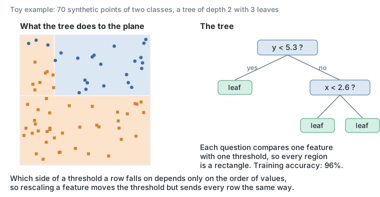
Figure 1. A toy example on 70 synthetic points. Each question compares one feature with one threshold, so the tree cuts the plane into rectangles.

CART

• CART is a greedy algorithm. At the top, it picks the split that improves the fit most right now, then repeats inside each child. It does not check whether a worse split now would allow better splits several levels down.
• A greedy algorithm often gives a reasonably good solution, but not a guaranteed optimal one.
• Finding the optimal tree is NP-complete, meaning no known method solves it quickly as the data grows, so practical algorithms settle for the greedy answer.

Decision trees challenges: regularizing

• Decision trees are nonparametric models: they can overfit by adapting too closely to the training data.
• Regularization limits the tree’s complexity with hyperparameters. In scikit-learn they are max_depth (how many questions deep), min_samples_split (rows a node needs before it may split), min_samples_leaf (rows each leaf must keep), max_leaf_nodes (how many leaves in total) and max_features (how many features each split may look at).

Decision trees challenges: orthogonal boundaries

• Decision trees create orthogonal decision boundaries, which makes them sensitive to data rotation.

A tree can only cut along one feature at a time. When the true boundary between classes is diagonal, it needs a staircase of many splits to follow it. Rotated 45 degrees, the same boundary needs 8 leaves instead of one split.

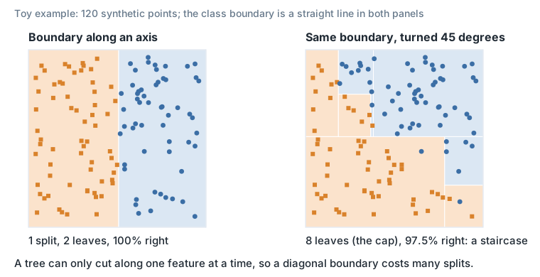
Figure 2. A toy example on 120 synthetic points. The same straight boundary takes one split along an axis, and a staircase of 8 leaves when turned, which still gets 97.5% of the points right.

Decision trees challenges: instability

• A single tree is easy to read, but trees are highly sensitive to small variations in the training data. The scikit-learn guide says: “small variations in the data might result in a completely different tree being generated”. A different first split changes every question below it.
• Random forests help with this instability by averaging the predictions of many trees.

Case study: max depth influence

On the weekly sales series, a single tree gave these errors, measured as WAPE (weighted absolute percentage error: total absolute error divided by total actual sales, lower is better) and indexed to the depth-1 tree = 100:

Here the deepest tree did best.

Ensemble methods

Bagging or pasting

• If several models make errors that differ, averaging them cancels part of those errors. So the models need to be independent enough that their errors are not the same.
• One way to make them differ is to train each one on a different random sample of the rows.
• Bagging (bootstrap aggregating) draws each sample with replacement, so a tree sees some rows twice and misses others.
• Pasting draws without replacement. Breiman proposed it for data too large to fit in memory: grow each predictor on a small piece, then combine them, and he reported accuracy comparable to what all the data held in memory would have given. The scikit-learn ensemble guide uses these names.
• Out-of-bag (OOB) evaluation: the rows a bootstrap sample leaves out are called out-of-bag. Each row can be predicted by the trees that never saw it, and scoring those predictions gives a validation estimate without a separate split; in scikit-learn this is oob_score=True.

The chance that a given row is never drawn in n draws is (1 − 1/n)^n, which approaches 1/e, about 37%, as n grows.

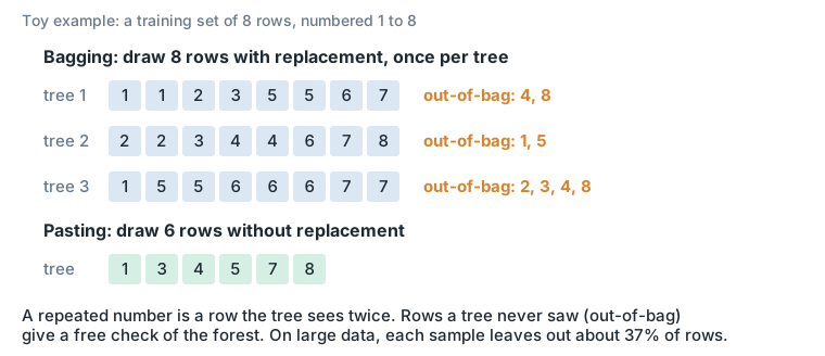
Figure 3. A toy example with 8 rows. Bagging repeats some rows and leaves others out; pasting never repeats a row. Rows a tree never saw (out-of-bag) give a free check of the forest.

Random forest

• A random forest is an ensemble of decision trees trained independently via bagging. In scikit-learn it is RandomForestClassifier or RandomForestRegressor.
• It adds extra randomness: each split only considers a random subset of the features. The scikit-learn guide explains the purpose: single trees have high variance, the randomness makes their errors partly independent, and averaging lets some errors cancel, sometimes at the cost of a little more bias.
• It has a built-in feature importance: how much each feature’s splits reduced the impurity (the loss inside a node). The scikit-learn guide warns that this measure is computed on training data and favours features with many unique values, and suggests permutation importance as an alternative.

Case study: random forest

On the same series, going from 5 trees (n_estimators=5) to 100 trees cut the random forest’s error by about 9%. More trees helped, but here the forest still had about 28% more error than the single deep tree above.

Gradient boosting

Boosting and GBM

• Boosting combines weak learners into a strong one by training predictors sequentially, each one correcting the errors of the ones before it.

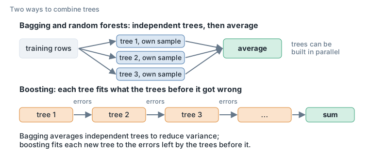
Figure 4. Bagging averages independent trees to reduce variance; boosting fits each new tree to the errors left by the trees before it.

• The two main models of boosting are AdaBoost and gradient boosting.
• AdaBoost reweights the rows: after each round, the rows the model got wrong weigh more, so the next learner concentrates on them.
• Gradient boosting fits each new tree to the negative gradient of the loss. The gradient says how the loss changes when a prediction moves, so its negative is the direction that lowers the loss fastest; for squared error it is simply the residual: actual minus predicted.
• XGBoost and LightGBM are both gradient-boosting libraries.

Some gradient boosting hyperparameters

• learning_rate scales the contribution of each tree, a technique Friedman called shrinkage. The scikit-learn guide notes that smaller rates need more trees to reach the same training error, and that small rates tend to give better test error.
• To control how many trees you build, use early stopping and an evaluation set. Too many trees eventually fit noise, so watch the error on a validation set and keep the round where it was lowest.

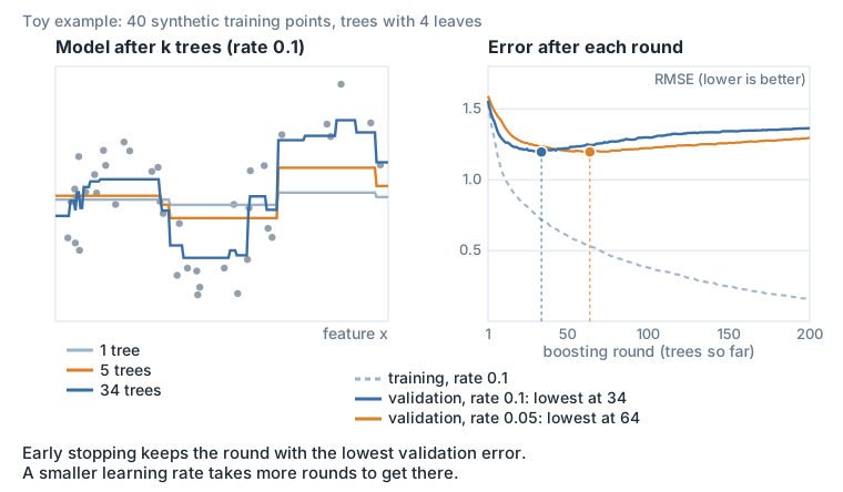
Figure 5. A toy example on 40 synthetic points. Validation error is lowest at round 34 with a learning rate of 0.1, and at round 64 with 0.05.

LightGBM

Motivation

From the LightGBM paper (Ke et al., 2017):

• To address the efficiency and scalability limits of existing GBDT implementations on large, high-dimensional data.
• To avoid scanning every row for every feature when calculating split points.
• To be faster than XGBoost while keeping comparable accuracy, as the paper’s experiments show.

LightGBM uses four techniques: leaf-wise growth, histograms, GOSS and exclusive feature bundling.

Leaf-wise tree growth

• Most tree learners grow level by level. LightGBM grows leaf-wise: at each step it splits the one leaf whose split lowers the loss most, wherever it is, so the tree grows deeper where the loss is high.
• With the same number of leaves, this tends to reach a lower loss, but it can overfit on small data, so it needs regularization. The main size control is num_leaves, backed by min_data_in_leaf and, if needed, max_depth.

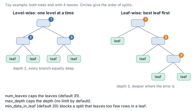
Figure 6. A toy example. Both trees have four leaves; the leaf-wise one is deeper where the error is.

Histogram based splitting

Problem:

• A pre-sorted learner tries the gap between every pair of neighbouring values of every feature.
• Pre-sorting is memory-intensive and computationally expensive.

Solution:

• LightGBM first puts each feature into at most max_bin bins (255 by default), with edges placed so that bins hold similar numbers of rows. This is done once, when the dataset is built, and the bins are reused across trees.
• During training it only adds up the gradients per bin and tries the bin edges as thresholds.
• Histograms for different features are independent, so LightGBM builds them in parallel across CPU cores.
• A leaf’s histogram can also be computed as its parent’s minus its sibling’s, so only the smaller child is built from the rows.
• Only bin values are stored, as small integers: one byte each when max_bin is 255.

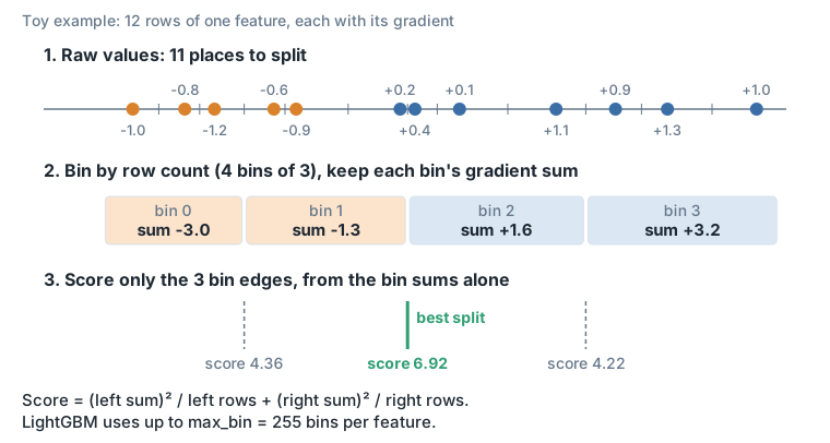
Figure 7. A toy example. Three bin edges are scored instead of eleven gaps.

Gradient based one side sampling (GOSS)

Problem:

• In ordinary gradient boosting, every training row is used to find the best split.
• Rows with larger gradients, the ones the model gets most wrong, have the larger effect on the split.

Solution:

• GOSS keeps the rows with the largest gradients and samples the rest. It keeps the top a share of rows by gradient size, draws a random sample the size of a b share of all rows from the others, and counts each drawn row (1 − a) / b times so their total weight stays about right.
• In LightGBM it is off by default; since version 4.0 it is chosen with data_sample_strategy="goss", with top_rate=0.2 and other_rate=0.1.

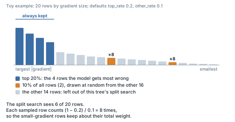
Figure 8. A toy example with LightGBM’s default rates.

Exclusive feature bundling

Problem:

• Sparse data, such as one-hot columns, often has columns that are rarely non-zero on the same row.
• Each of those columns still needs its own histogram.

Solution:

• Exclusive feature bundling merges such columns into one column and gives each original its own range of bins, so the values stay distinguishable.
• Finding the best bundling is NP-hard, so the paper uses a greedy approximation, optionally allowing a little overlap.
• This cuts histogram construction time, which is proportional to rows × features, to rows × bundles.
• LightGBM bundles by default.

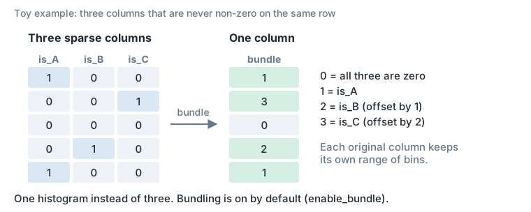
Figure 9. A toy example. One histogram replaces three.

In the paper’s five benchmarks, adding GOSS and bundling to LightGBM’s own histogram algorithm cut training time per iteration by 1.6 to 21 times, with almost the same accuracy.

Hyperparameters

LightGBM’s parameters split into the modeling setup (objective, boosting), those that control the ensemble training, such as the number of trees and the learning rate, and those that control the growth of each tree, such as max_depth and min_data_in_leaf.

Modeling setup

Objective, for regression:

• regression (L2, squared error): the default; aims at the mean.
• regression_l1 (L1, absolute error): aims at the median and is less sensitive to outliers than squared error.
• quantile: predicts a chosen quantile instead of the mean, which can be used to build prediction intervals.
• poisson and tweedie: use a log link and fit non-negative targets such as counts. With a variance power between 1 and 2 (LightGBM’s default is 1.5), the Tweedie distribution puts a point mass at zero and is continuous above it.
• gamma and mape are also available.

Boosting:

• gbdt by default, or dart. DART is a variant that leaves out a random subset of the earlier trees when working out what the next tree should fit, an idea borrowed from dropout in neural networks.
• The tuning guide lists “Try dart” under better accuracy. It is slower per round: LightGBM’s DART code subtracts the dropped trees from the running predictions and adds them back rescaled. Early stopping does not apply to it.

Tree growth parameters

• max_depth: controls the degree of feature interactions, by limiting how many features one path from root to leaf can combine.
• min_data_in_leaf: the minimum number of rows in a leaf.
• num_leaves: the number of leaves in a tree.
• min_gain_to_split: the minimum gain to consider splitting a node.
• lambda_l1 and lambda_l2: in a linear model, L1 and L2 regularization apply to the feature coefficients. In LightGBM they apply to the leaf values. In LightGBM’s source, a leaf’s value is minus its summed gradient divided by its summed second derivative plus lambda_l2, so lambda_l2 pulls every leaf toward zero. lambda_l1 first shrinks the summed gradient toward zero by lambda_l1, so a leaf with a small summed gradient gets a value of exactly zero. Unlike L1 in a linear model, it does not drop features.

Ensemble related parameters

• learning_rate and the number of trees: a low learning rate needs more trees, and tends to generalize better.
• bagging_fraction: the share of rows used for each tree (subsample in XGBoost).
• bagging_freq: how often the rows are resampled. A bagging_fraction below one has no effect while bagging_freq is 0.
• feature_fraction: the share of features randomly chosen for each tree (colsample_bytree in XGBoost).
• Smaller row and feature fractions also make training faster.

Recommendations

Start by defining the problem: the objective. Then, from LightGBM’s parameter-tuning guide:

For better accuracy:

• Use large max_bin (may be slower).
• Use small learning_rate with large num_iterations.
• Use large num_leaves (may cause over-fitting).
• Use bigger training data.
• Try dart.

To deal with over-fitting:

• Use small max_bin and num_leaves.
• Use min_data_in_leaf.
• Use bagging by setting bagging_fraction and bagging_freq.
• Use feature sub-sampling by setting feature_fraction.
• Try lambda_l1, lambda_l2 and min_gain_to_split for regularization.
• Try max_depth to avoid growing deep trees.

The deck’s LightGBM case study, hand-tuning the same series, is in the tuning post, with how far tuning is worth taking.

Categorical features vs continuous features

• LightGBM does not convert categories to one-hot encoding internally. The usual way to feed a category to a model is one-hot encoding: one 0/1 column per category. LightGBM’s features page calls this suboptimal for trees: with many categories, a tree built on one-hot columns tends to be unbalanced and has to grow very deep.
• Instead, LightGBM takes the category as one integer column (non-negative codes; negative values are treated as missing) and splits it by dividing the categories into two groups.
• Each category gets its own bin in the histogram, holding that category’s gradient sums; very rare categories can be left without one, as the binning code shows.
• A rule might read “categories 1, 3 and 5 go left, 0, 2 and 4 go right”. This is different from how continuous features are split.
• With k categories there are 2^(k−1) − 1 ways to divide them, too many to try. LightGBM follows a result by Fisher (1958): sort the categories by their sum of gradients divided by their sum of second derivatives (how fast the gradient itself changes; for squared error, simply the number of rows), then try only the cuts along that order. That takes about k log k steps.

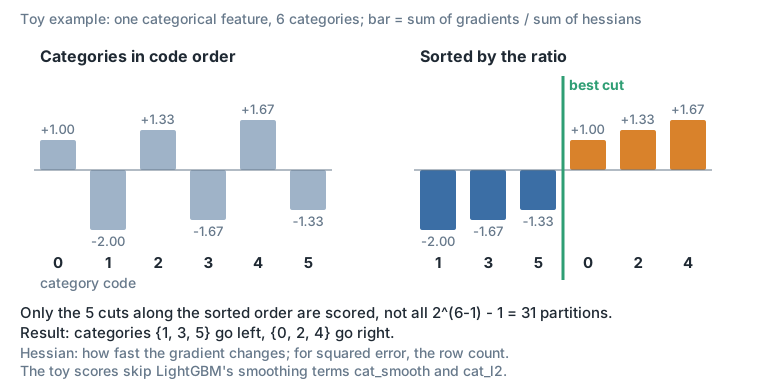
Figure 10. A toy example with six categories. Five cuts are scored instead of 31 partitions.

Key hyperparameters for categorical features

• max_cat_to_onehot (4 by default): with at most this many categories, LightGBM uses a simpler one-versus-rest split.
• max_cat_threshold (32): limits how many split points are considered.
• cat_smooth (10): reduces the effect of noise in categories with few rows.
• cat_l2 (10): adds L2 regularization to categorical splits.
• min_data_per_group (100): the minimum rows per category group.

References

• Ke et al., “LightGBM: A Highly Efficient Gradient Boosting Decision Tree”, NeurIPS 2017.
• LightGBM, features overview, parameters, parameter-tuning guide, the leaf-value code and the DART code.
• scikit-learn user guide, decision trees and ensembles.
• Quinlan, “Induction of Decision Trees”, 1986.
• Hyafil and Rivest, “Constructing Optimal Binary Decision Trees Is NP-Complete”, 1976.
• Breiman, “Bagging Predictors”, 1996; “Pasting Small Votes for Classification in Large Databases and On-Line”, 1999; “Random Forests”, 2001.
• Freund and Schapire, “A Decision-Theoretic Generalization of On-Line Learning and an Application to Boosting”, 1997.
• Friedman, “Greedy Function Approximation: A Gradient Boosting Machine”, 2001.
• Rashmi and Gilad-Bachrach, “DART: Dropouts meet Multiple Additive Regression Trees”.
• Fisher, “On Grouping for Maximum Homogeneity”, 1958.
• Rob J. Hyndman, “WAPE: Weighted Absolute Percentage Error”.