Explainability Using SHAP

Intro

Model predictions are only as valuable as our ability to understand them. SHAP solves this by decomposing any prediction into the contribution of each input feature, giving us both global feature importance and local instance-level explanations.

The key insight: every prediction can be written as base_value + sum(SHAP_values), where each SHAP value represents how much a feature pushed the prediction above or below the expected model output. This additive property makes SHAP values interpretable and comparable across features.

You’ve trained your model and it works. Now you need to understand why. SHAP decomposes predictions into feature contributions, but the real insight comes from proper visualization.

This post walks through the essential SHAP visualizations and analysis techniques using our forecasting model, showing how to move from basic feature rankings to sophisticated pattern discovery in your data.

The model is a LightGBM model that forecasts weekly sales. Feature names are replaced by generic ones (category level 1 to 4 are the levels of the product hierarchy, from the broadest to the finest), and every SHAP value in the figures is indexed: 100 is the mean absolute SHAP value of the model’s strongest feature, unless the figure says otherwise.

How SHAP computes the values

SHAP values are the Shapley values of a conditional expectation of the model’s output: a feature’s SHAP value is the change it makes to the expected prediction when it is added, averaged over every order in which the features can be added (Lundberg and Lee, 2017). The base value is the prediction expected when no feature is known, E[f(X)].

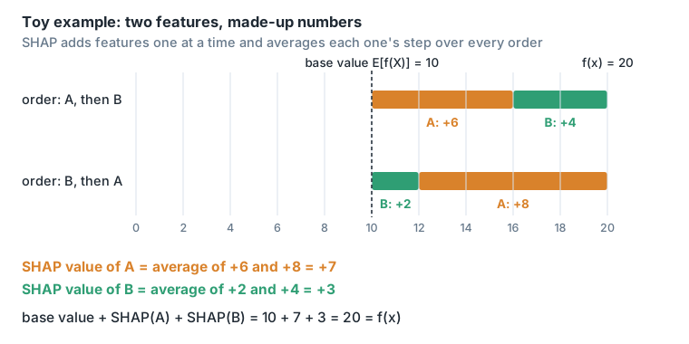
For tree models, TreeSHAP computes these values exactly in polynomial time instead of exponential time (Lundberg, Erion and Lee, 2018). shap.Explainer(lightgbm_model, masker=None) picks it, and with no background data it uses the number of training rows that went down each branch to stand for the missing features.

N.B.: since our model is using a Tweedie objective, f(x) represents the log of the model’s prediction. SHAP explains the output of the tree model directly; the model’s final result is exp(result of the tree structures). The result of the tree structures can be found with internal_model.predict(inference_ds, raw_score=True).

So the SHAP values add up in log space, and exp(SHAP value) is the factor by which a feature multiplies the forecast. LightGBM’s Tweedie objective uses a log link.

Plots

Bar plot

lgb.plot_importance(lightgbm_model, importance_type="gain")

gives a similar ranking to

shap.plots.bar(shap_values)

Both put the same feature first, but the order below it differs. Gain counts how much the splits on a feature reduced the loss during training (LightGBM docs); the SHAP bar plot shows the mean absolute SHAP value over the rows being explained.

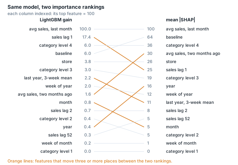
But in SHAP you can also show the feature that most impacted the result using the max value of shap_values:

shap.plots.bar(shap_values.abs.max(0))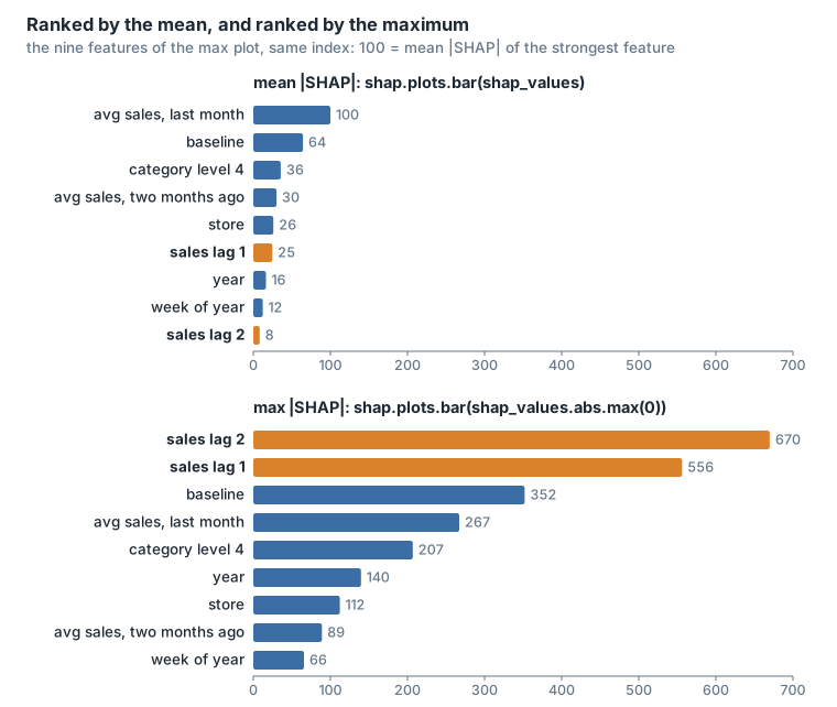

Heatmap plot

Shows SHAP values across all samples simultaneously. Each row is a feature, each column a sample, color shows the contribution.

shap.plots.heatmap(shap_values, max_display=12)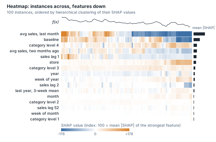

The line above the heatmap is the model output f(x), and the bars on the right are each feature’s mean absolute SHAP value. By default the samples are ordered by a hierarchical clustering of their SHAP values (shap docs).

NB: takes a lot of time, choose 100 samples or less.

Beeswarm plot

The beeswarm plot provides a global overview of SHAP values for selected features, with rows representing each feature ranked by the mean absolute SHAP value. The individual dots in each row are the SHAP values for that particular feature in each sample of the dataset.

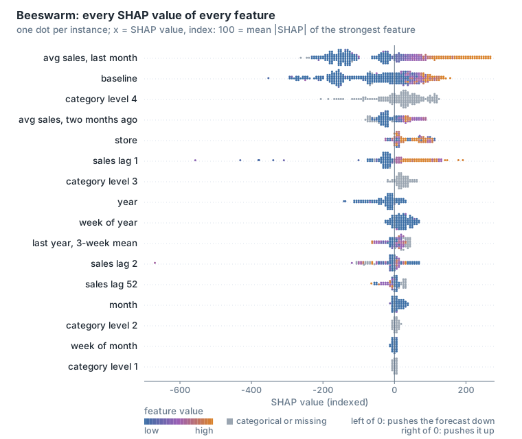
The colour of a dot is the feature’s value in that sample, from low (blue) to high (orange); categorical features and missing values are grey.

By default SHAP uses the mean absolute value of shap_values to order the features in a beeswarm plot from most important (at the top) to the least important. We can choose to do the ordering based on the max instead of the mean:

shap.plots.beeswarm(shap_values, order=shap_values.abs.max(0))

Scatter plot

Shows interaction between features.

shap.plots.scatter(shap_values[:, "baseline"], color=shap_values)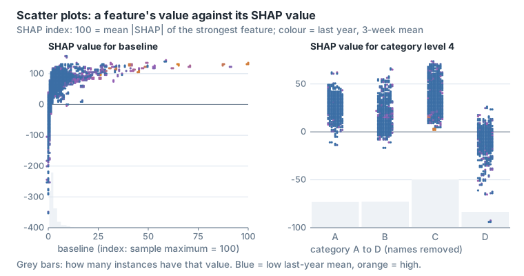

The x axis is the feature’s value and the y axis its SHAP value; the grey bars are a histogram of the feature’s values.

You can either choose the color feature or let SHAP determine the one with the strongest interaction effect with your main feature (baseline). This is calculated using shap.utils.approximate_interactions().

Example of an analysis

Using the bar plot with the max component we got the max bar plot in the Bar plot section, which shows that sales lag 1 and 2 are the features that affect the model the most.

To get an even richer representation showing all the distribution of the shap_values for any given feature (not just the mean and max) we can use:

shap.plots.beeswarm(shap_values.abs, color="shap_red")

Here we can see clearly that although the mean SHAP values of sales lag 2 and sales lag 1 are not the most important amongst features, their max values are. Which means that in some specific cases they sway the model a lot. What are those cases?

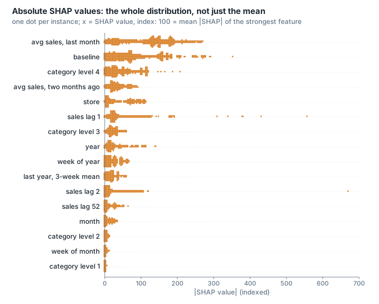
To get a double sided distribution we can use:

shap.plots.beeswarm(shap_values, max_display=20)

This allows us to see that sales lag 1 and sales lag 2 most strongly impacted the model to reduce its prediction value (the beeswarm plot in the section above).

We can for example examine the case where the sales lag 1 SHAP value is at its min:

lag1 = shap_values[:, "sales_lag_1"].values
index_min_lag_sales1 = np.where(lag1 == np.min(lag1))[0][0]

Then we plot the explainability for that specific case:

shap.plots.bar(shap_values[index_min_lag_sales1], max_display=20)

and we get:

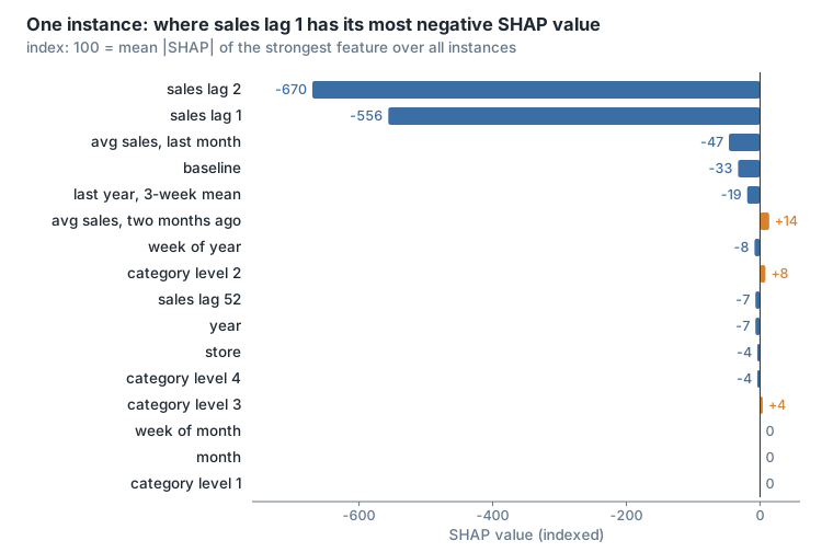
To see how that compares to the max and average SHAP value of sales lag 1, we can do the following (index_max_lag_sales1 is found the same way, with np.max):

val = ["max" if i == index_max_lag_sales1 else "min" if i == index_min_lag_sales1 else "other"
       for i in range(len(lag1))]
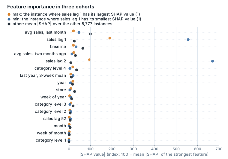
shap.plots.bar(shap_values.cohorts(val), max_display=20)

In this plot we can for example see that when sales lag 1 and 2 are at their max or min SHAP values, the importance of the other features to the model prediction is very small; when they’re at their average value, the importance of baseline and average sales last month increases significantly.

Or let SHAP choose the cohorts that best separate the data. In the plot below we let SHAP split the data into the 5 most homogeneous groups using:

shap.plots.bar(shap_values.cohorts(5).abs.mean(0))

SHAP fits a decision tree with 5 leaves on the feature values to separate the SHAP values, and each leaf is a cohort.

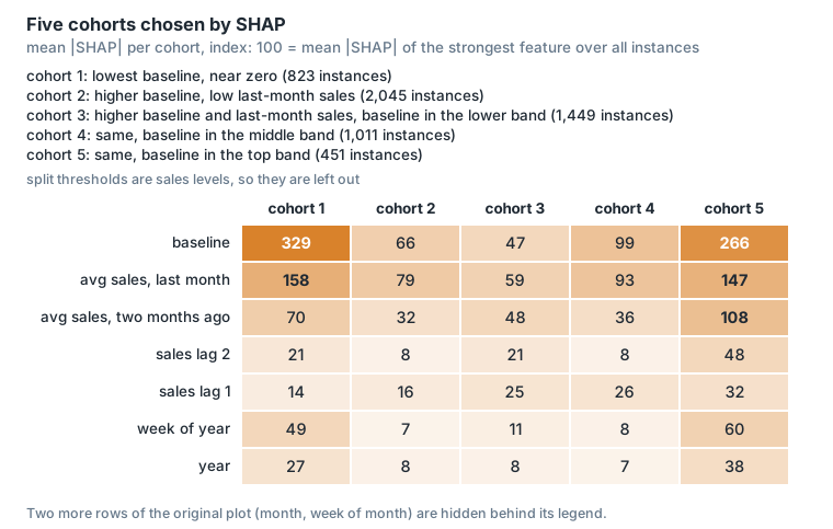
This gives us some ideas about the different groups of patterns inside our data.

Features correlation using SHAP

Often features in datasets are partially or fully redundant with each other. Where redundant means that a model could use either feature and still get the same accuracy. (This text follows the shap bar plot documentation.)

To find these features we often compute correlation matrices among the features, or use some type of clustering method. SHAP offers a more direct approach that measures feature redundancy through model loss comparisons. The shap.utils.hclust method can do this and build a hierarchical clustering of the features by training XGBoost models to predict the outcome for each pair of input features.

For a typical tabular dataset this results in much more accurate measures of feature redundancy than you would get from unsupervised methods like correlation.

The algorithm:

1. Train univariate XGBoost: feature i → y
2. Train cross-prediction: feature j → feature i’s predictions
3. If j predicts i’s output well, they’re redundant
4. Build distance matrix, apply hierarchical clustering

# trains one single-feature XGBoost model per feature,
# then one per ordered pair of features (step 2)
clustering = shap.utils.hclust(X, y)
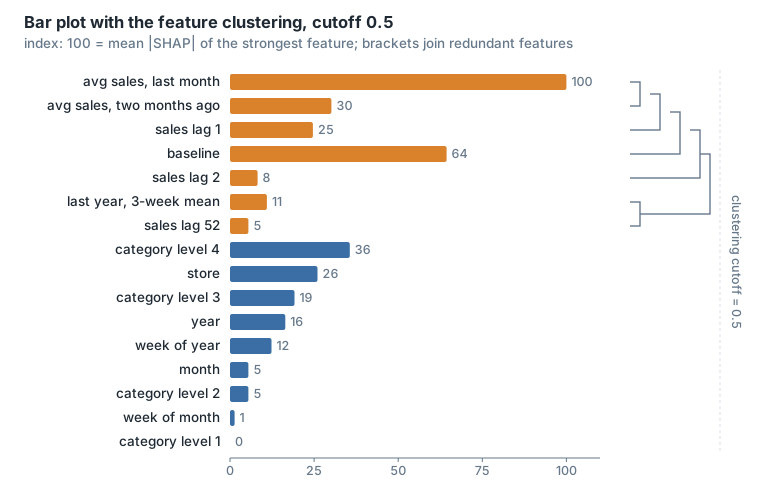
shap.plots.bar(shap_values, clustering=clustering, clustering_cutoff=0.5)

By default clustering_cutoff is 0.5, meaning we only group features that have a distance < 0.5 (they are more than (1 - clustering_cutoff) similar). The distance is 1 minus the share of variance that feature j’s model explains of feature i’s predictions (shap source).

For our case we can see that we have strong correlation between most of the calculated lag features, using a clustering_cutoff of 0.5.

Template notebook

The template notebook (explainability minimalist base) runs the same steps on any slice of the data. Its model is a LightGBM model with a Tweedie objective (variance power 1.6, 256 leaves, learning rate 0.05, at least 300 rows per leaf, L1 and L2 regularisation of 3, 80% bagging and feature fraction, 3,000 iterations), one model per forecast horizon; the notebook explains horizon 1. Its features are calendar features (month, year, week of month, week of year, weeks to the next and previous holiday), categorical features (store, category level 1, category level 4, country, product type, colour, store format, previous and next holiday, price type) and numeric ones (baseline, average sales last month, item business weight, price, price coefficient), plus last year’s 3-week mean for the horizon, and sales lag 1 for horizons below 4.

Its functions:

• load_explain: filters the data to one slice, loads the model, computes the SHAP values with shap.Explainer(model, masker=None), draws the beeswarm plot, draws a cohort bar plot for every categorical feature with 2 to 9 values, then clusters the features with shap.utils.hclust (categorical features label-encoded, and the model’s own prediction as y) and draws the clustered bar plot at cutoffs 0.2, 0.3, 0.4 and 0.5.
• plot_cohorts_feat: one cohort per value of a categorical feature, drawn with shap.plots.bar on shap_values.cohorts(labels).
• remove_nan_shap: keeps the rows where one feature, or every feature, has a value.
• analyze_behaviour: splits the rows with a condition on the feature values or on the SHAP values, plots the cohort’s mean absolute SHAP against the other rows, finds the 3 features whose mean absolute SHAP differs most between the two (in %), and plots the histograms of those features’ values for both groups.

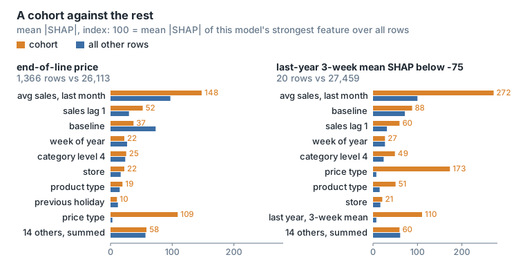
analyze_behaviour(shap_values, "data", "price_type == 'end_of_line'", description="behaviour")
analyze_behaviour(shap_values, "values", "last_year_3week_mean < threshold", description="behaviour")

On one country’s rows, the beeswarm ranks average sales last month first, then baseline, sales lag 1, week of year and category level 4.

For the rows with an end-of-line price, price type has a mean absolute SHAP 3826.7% larger than for the other rows. The next two features are the price coefficient (280.5%) and sales lag 1 (78.1%). In the price coefficient histogram, for end-of-line rows it is spread below 1, while for the other rows it is almost always 1.

For the 20 rows where last year’s 3-week mean has a SHAP value below -75 on the index of the figure, the largest differences are price type (2096.4%), last year’s 3-week mean (1302.7%) and week of month (262.8%). Most of these rows have an end-of-line price, and their last-year 3-week mean is higher than for the other rows. Week of month has the same value in both groups, so its difference comes from the SHAP values, not from the data.

The cohort plots per categorical feature show:

• store format: the two formats give almost the same importances; store is a little more important in the format with fewer rows.
• price type: price type matters for end-of-line rows, less for promotion rows, and almost not for standard prices. In the rows where the price type is missing, baseline and price matter far more than in any other price type.

The feature clustering of this model, at the four cutoffs:

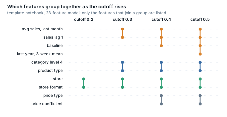
Features that are constant inside the slice (for example country, when the slice is one country) get no signal in hclust, which warns and sets all their redundancy distances to 1.

Explainability dashboard

A demo of an explainability dashboard, built for a different model (its features differ from the ones above), in two parts.

1. Select a feature and its activity.
   • Controls: the model variant, the target horizon, the feature to inspect, the contribution direction (for example largest negative effect), the units of the SHAP ranking (model sales units) and the high-activity cohort (for example the top 1% of rows by that feature’s contribution).
   • Feature value → SHAP contribution: a scatter of the feature’s input value against its SHAP value, with the high-activity rows highlighted. Missing inputs are excluded only from the x axis and histograms, never from the SHAP ranking.
   • High-activity cohort vs remaining rows: mean absolute SHAP of every model feature, top 15, for the cohort and for the other rows. This comparison is descriptive: the cohort was chosen using this feature’s contribution.
2. Strongest examples, with a matched baseline comparison.
   • Pick one of the top 3 examples in the selected direction, or go to the next one.
   • A waterfall of the example’s forecast over all 24 features, with the inspected feature in bold (here the recent versus last year ratio). Waterfalls always use raw model/store units, before clipping and rounding.
   • The history of the series, the forecasts of the model and of the baseline, and the actuals, around the forecast cutoff. Actuals are not used in the ranking.

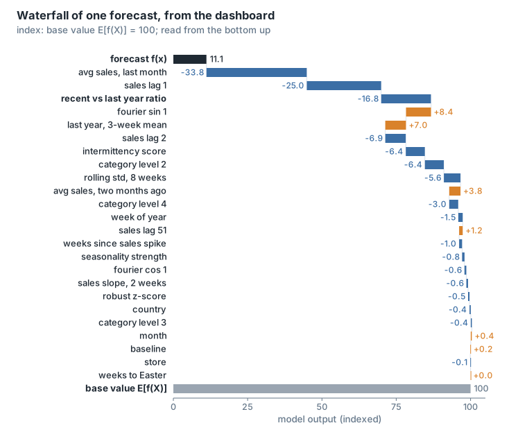
The model behind the dashboard predicts a normalised target (sales minus a mean, divided by a standard deviation; the dashboard prints both for each example), so the dashboard multiplies each SHAP value by that standard deviation to show it in sales units. The contributions still add up: base value plus the 24 contributions equals the forecast.

Sources

• Scott Lundberg and Su-In Lee, A Unified Approach to Interpreting Model Predictions, NIPS 2017.
• Scott M. Lundberg, Gabriel G. Erion and Su-In Lee, Consistent Individualized Feature Attribution for Tree Ensembles, 2018.
• shap documentation: bar, beeswarm, heatmap and scatter plots; the feature-redundancy text above follows the bar plot page.
• shap source, shap/utils/_clustering.py (hclust and xgboost_distances_r2).
• LightGBM documentation: parameters and plot_importance.