These studies are part of a series of experiments aimed at improving the way we design our models, in particular by investigating the introduction of an evaluation set, the choice of optimal hyperparameters for the models, and the selection of a relevant and reasonable feature set. The model is a LightGBM model that forecasts weekly sales per item and store, with one model per product category x zone. The results are shown relative to a baseline model, as a difference in points (or, in one figure, an index where the baseline is 100), not as absolute values.
The bias seen in these studies, under-forecasting high sellers and over-forecasting low sellers, is the subject of the next post.
Validation Set Study
Summary of findings
This study aimed to determine the most effective validation set strategy for early-stopping in our forecasting models, while preparing the ground for upcoming hyperparameter optimization and feature selection experiments. Five methods were evaluated across various product categories, zones, and cutoffs, using a fixed set of hyperparameters and the current production feature set, supplemented with all newly added features (covering SKU, BU, holidays, and price characteristics).
Results show that all evaluation set methods deliver similar or slightly better forecasting performance (≈ 2% WAPE improvement at horizon 4) compared to the production baseline, with the gain being more pronounced for lower selling classes (0 and 1). The last_year_exclusive_True method stands out slightly, triggering early stopping more often than the other methods and reducing training rounds, and thus lowering computation time while maintaining decent accuracy. Bias differences were generally small, with no method clearly outperforming across all horizons and product categories.
Given the marginal but consistent advantages and potential time savings, last_year_exclusive_True is recommended as the default approach moving forward.
Intro
A first study has been led to find the best validation set for an early-stopping training strategy. It is illustrated in the diagram below:
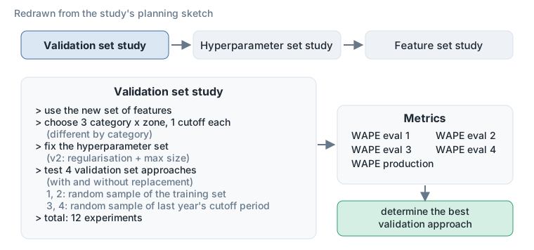
Figure 1. The series of studies, and the validation set study’s plan, redrawn from the study’s sketch.
Setup of the Experimentation
We would like to investigate 4 different strategies for evaluating the error during training. These are listed below:
- random_exclusive_False: random sampling on training dataset (validation set included in training set)
- random_exclusive_True: random sampling on training dataset (validation set excluded from training set)
- last_year_exclusive_False: random sampling on training dataset over last year’s cutoff period (validation set included in training set)
- last_year_exclusive_True: random sampling on training dataset over last year’s cutoff period (validation set excluded from training set)
- none_exclusive_False: no specific validation set, the validation set is taken to be the training set (which allows us to observe the evolution of the training loss)
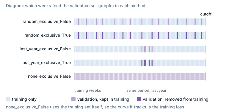
Figure 2. Which weeks feed the validation set in each method. A diagram, not data.
We conducted this experiment on the following perimeter:
- 3 variations of product categories (small, medium and large) and cutoffs:
- a large product category x zone, with one cutoff
- a medium product category x zone, with a cutoff before Christmas
- a small product category x zone, with a cutoff with no holiday
- set of features: the production model’s, below
- a fixed set of hyperparameters, defined below
Fixed set of hyperparameters
We fixed a set of hyperparameters in the middle of what we want to experiment with as hyperparameters.
num_leaves was first fixed at 131072 as planned, however this resulted in very slow training of the model (3.5h for 100 training rounds). We therefore decided to revert back to 256 for the purposes of the validation set experimentation.
| Hyperparameter | Production | Fixed for this study |
|---|---|---|
| objective | tweedie | tweedie |
| tweedie_variance_power | 1.6 | 1.6 |
| boosting | gbdt | gbdt |
| bagging_freq | 1 | 1 |
| bagging_fraction | 1 | 0.9 |
| feature_fraction | 0.8 | 0.8 |
| learning_rate | 0.07 | 0.07 |
| max_depth | 256 | -1 |
| num_leaves | 1024 | 256 |
| min_data_in_leaf | 100 | 50 |
| num_iterations | 1000 | 1000 |
Features
The features used represent the production features plus the preselection of features we added. The number of features evolves from 17 to 44:
- Integer features: month, year, week of month, week of year, count of exceptional open days, count of exceptional closed days, number of holidays in the week, on weekdays and on weekends, number of weeks to the next holiday and since the previous holiday.
- Categorical features: store, country, product family, sub-department, department, product category, brand, product technicity level, product nature, product nature category, colour, region, store category, price type, first holiday name, next holiday name, previous holiday name, holiday in week (flag), worked day in week (flag).
- Float features: baseline quantity, average sales last month, average sales two months ago, last year’s 3-week centred mean for the horizon, the last-year lag (53 minus the horizon), lag 1 and lag 2 (if horizon < 4), item business weight, display price, reference price, price coefficient for the period, reference coefficient, price coefficient all time, count of open days in the week.
Detailed Results
Comparison of early stopping results
For each perimeter we run all 5 methods, here are the average times it took for a run on each perimeter.
| Perimeter | Average duration (minutes) | Training size (rows) |
|---|---|---|
| small | 8.6 | ~ 900 K |
| medium | 35.4 | ~ 20 M |
| large | 92.6 | ~ 60 M |
Number of models trained = number of perimeters x number of methods x number of horizons = 3 x 5 x 8 = 120.
Default training rounds: 1000.
We run each validation set method on 3 perimeters, below is the total and average number of training rounds of experiments for the total number of models.
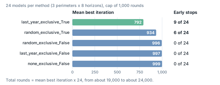
Figure 3. Mean best iteration and number of early stops, per method. The mean RMSE of each method is left out: each is calculated on a different validation set, so direct comparison isn’t viable.
Advantages of using a validation set:
- Monitor model performance: track validation loss during training
- Early stopping: training stops before 1000 rounds if validation error starts degrading, which:
- Prevents overfitting
- Reduces training time
- Optimal model selection: if training completes all 1000 rounds, the best performing model (by validation score) is still selected
- Resource optimization: save computational resources by stopping ineffective training early. Therefore allowing us to experiment with more training rounds (5000) to squeeze more performance from the model.
In conclusion, last_year_exclusive_True is the method that triggers early stopping and reduces the number of training rounds the most. When exclusive is False, we tend to overfit more by reducing RMSE further, which can lead to better accuracy if the model naturally underfits but runs the risk of overfitting otherwise. However, exclusive = False never triggered early stopping.
Comparison in metrics by selling class
For the simplification, we focus on one country in the analysis of results for the large and medium perimeters. Forecasts are compared to raw sales data to compute metrics.
WAPE 4: in terms of WAPE at horizon 4, the different methods using the evaluation set deliver similar results and outperform the baseline (production). Overall, we observe a 2% WAPE improvement, which is even more pronounced for selling classes 0 and 1. The “last_year_exclusive_False” method appears to stand out, showing a slight advantage for selling class 0, but gives similar results to other new models for the remaining selling classes.
Bias 4: from a bias perspective at horizon 4, the results are also similar for both lower and higher selling classes. The production model’s performance is also lower than that of the new methods. However, it is worth noting that at horizon 8, the production model appeared to perform better overall, due to the compensation between over-forecasts in lower selling classes and under-forecasts in higher selling classes.
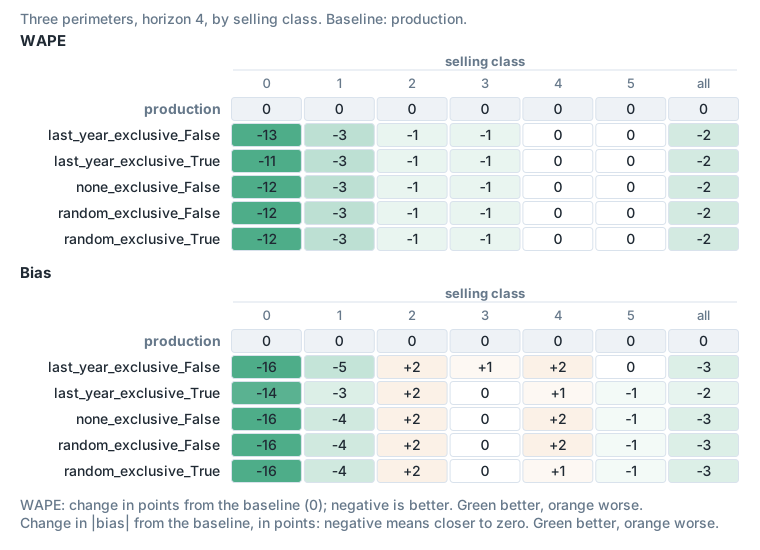
Figure 4. WAPE and bias at horizon 4 by selling class, relative to production.
Comparison in metrics by product category
WAPE 4: the WAPE at horizon 4 highlights the same previous observations: the “last_year_exclusive_False” method stands out with better performance, especially for the large product category (-2% WAPE compared to production) and the small product category (-5% WAPE compared to production). But we can notice that except for the small product category, the performances of all new models are similar.
Bias 4: on the other hand, in terms of bias at horizon 4, the “last_year_exclusive_True” method performs better on the small product category, while “last_year_exclusive_False” performs better on the large product category. Production still remains the best performer on the medium product category.
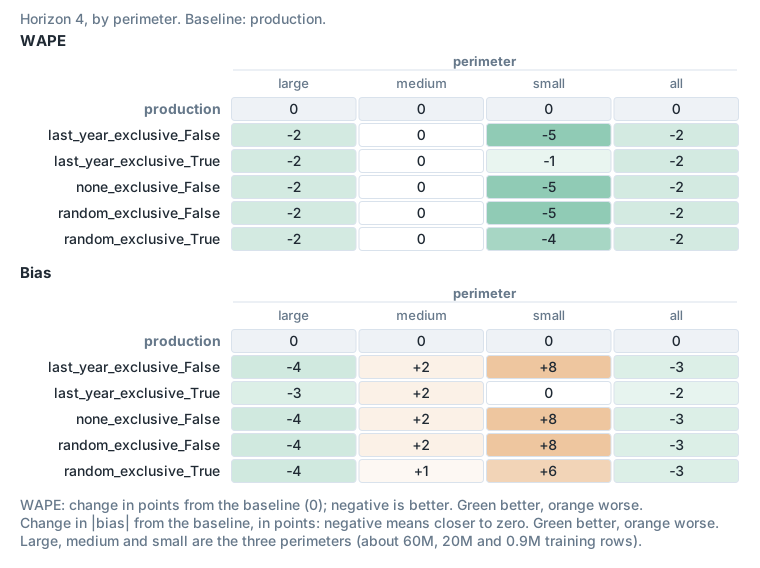
Figure 5. WAPE and bias at horizon 4 by perimeter, relative to production.
Conclusion
The different methods do not seem to stand out clearly in terms of WAPE or Bias. We recommend using the “last_year_exclusive_True” method, which comes slightly ahead and triggers early stopping the most often.
Annex: forecasts comparison for examples of time series
We compared the forecasts of the different models on examples of (sku, bu), selected on the WAPE at horizon 8 of last_year_exclusive_False: examples from the lowest and the highest WAPE, mixing high sellers and low sellers. They show single products’ weekly sales, so they are not reproduced here.
Annex: pre-hyperparameter experimentation study
Hyperparameters analysis
We analysed the model and extracted the tree structure for each tree for 2 models; the results are identical.
num_leaves:
- exactly 256 for each tree, which indicates that the model has an appetite for a higher number of leaves (in the production model, we fixed 1024 as the num_leaves; similarly all trees have exactly 1024)
- we increased this parameter to 8196 with 5000 as the number of rounds and we got exactly 8196 leaves for each of the 5000 trees. This training took 7h30 on average with last_year_exclusive_False and last_year_exclusive_True
- this parameter should be increased from 1024 but carefully (by counterbalancing it with min_data_in_leaf) since it will cause overfitting
min_data_in_leaf: we fixed this parameter at min_data_in_leaf = 50. Across all 1000 trees of this model, we observe 372 leaves out of 256000 with fewer than 50 examples.
This is normal behaviour. LightGBM checks min_data_in_leaf against a row count that it estimates from the sum of the hessians in each histogram bin, not against the exact count (source), so with an objective such as Tweedie, whose hessians differ from row to row, a leaf can end up with fewer rows than the limit.
For example, on a given model with min_data_in_leaf = 50, we found the following distribution of leaf sizes:
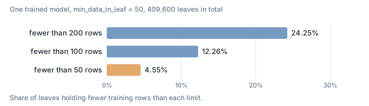
Figure 6. Leaf sizes in one model with min_data_in_leaf = 50, out of 409,600 leaves.
We propose to test the following hyperparameters during the next phase:
| Hyperparameter | Production | Proposed for the next phase |
|---|---|---|
| objective | tweedie | tweedie, mse, mae |
| tweedie_variance_power | 1.6 | 1.4, 1.6, 1.8 |
| boosting | gbdt | gbdt, dart |
| bagging_freq | 1 | 1 |
| bagging_fraction | 1 | 0.9 |
| feature_fraction | 0.8 | 0.8 |
| learning_rate | 0.07 | 0.07 |
| max_depth | 256 | -1 |
| num_leaves | 1024 | 4096, 8192, … |
| min_data_in_leaf | 100 | 10, 50, 100 |
| num_iterations | 1000 | 5000 |
| L1_regularization (optional) | 0.2, 0.5, 0.8 | |
| L2_regularization (optional) | 0.2, 0.5, 0.8 |
We’ll try to set num_leaves to the max that will not result in very long training time. Then we’ll vary the other parameters.
Annex: features analysis
Analysis on:
- subset 1, constituted of 2735 observations: one product family, one country, one cutoff, horizon 1
- subset 2, constituted of 14126 observations: one sub-department, the same country, cutoff and horizon
They show similar results; subset 2 is presented below unless otherwise specified. All analyses are subset bound: they apply to that specific subset and model used. Their generalization should be verified rather than assumed.
Beeswarm plot
The beeswarm plot provides a global overview of SHAP values for selected features, with rows representing each feature ranked by the mean absolute SHAP value. The individual dots in each row are the SHAP values for that particular feature in each sample of the dataset. For numerical features we can observe the following:
- for display price and reference price, the higher it is, the lower is the model’s prediction
- things are more complicated for price coefficients it seems, but the all-time price coefficient seems to show the clearest pattern of higher coefficient, lower prediction
- item business weight also contributes to the model’s prediction without a clear linear relationship
- for the rest of the numerical features (count of open days in the week, exceptional open and closed days, holidays in the week, on weekdays and on weekends, weeks to the next holiday and since the previous holiday), the importance to the model is very small for this subset, in part because there aren’t many holidays in this period in this country
For categorical features, these features seem to matter the most from the beeswarm plot: price type, region, colour, product nature, next and previous holiday name, product technicity level.
Importance plots for different cohorts
- price type: the price type feature has more importance when it’s not a standard price. However the other price features aren’t as polarizing as price type, so we should use the forecasting week’s price.
- product technicity level (subset 1): this feature matters the most to the model (in this subset) for high technicity, and the least when it’s least specific (all levels).
- product nature (subset 1): the strong correlation with price type is due to the fact that all 11 observations for one product nature have “end of line” as price type and their price has dropped by 18% (although that doesn’t seem to matter as much as price type to the model, e.g. the all-time price coefficient).
- brand and store category: cohort plots were also made; their cohorts are brand and store format names, so they are not reproduced.
Feature correlation
With a clustering cutoff of 0.7 (linking features that have a distance < 0.7) and of 0.3 (distance < 0.3):
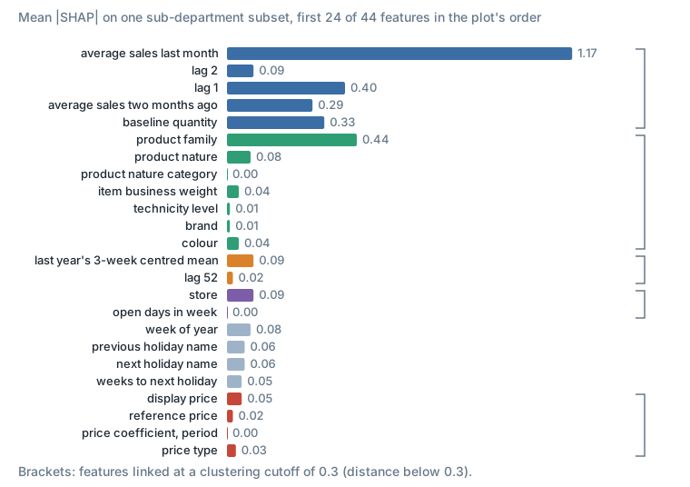
Figure 7. Mean |SHAP| per feature on subset 2, with the clusters at a cutoff of 0.3. SHAP values are in the model’s output units, not an accuracy metric.
More SHAP analysis will be conducted after phase 2 (hyperparameters experimentation).
Hyperparameter Set Study
Summary of findings
This study aimed to determine the most effective hyperparameters to support the change to our product category x zone modeling approach.
Our experimentations were conducted in a structured way (objective function, then complexity of tree, then regularization). First we tested many variations for each hyperparameter on one small perimeter to derive broad trends. We then proceeded by testing smaller variations of the hyperparameters on 3 perimeters.
Our analysis focused on understanding the effect of hyperparameters on models. We conducted several studies regarding the objective function and the fallacy of our evaluation metric, the potential for optimization for high sellers and the distribution of several key hyperparameters in the trained models.
We concluded the study by specifying 3 hyperparameter sets depending on the size of the cluster. The chosen hyperparameters reflect our key conclusions:
- Tweedie remains the optimal objective function for our problem, with a matching metric.
- More, less complex trees are better than fewer, more complex ones.
- A reasonable regularization allows better generalization of the models.
- Adapting learning rate and other hyperparameters to the cluster size is necessary.
We also uncovered many interesting facts about our models:
- We continue to observe a pattern of overforecasting low sellers and underforecasting high sellers. One model seems to be simply unable to optimize both behaviour predictions simultaneously.
- Tweedie loss, like WAPE loss, is higher for lower sellers than high sellers for a given constant error = y_pred - y_true. We need a better metric and we need to include it in the training process.
- We can tune the Tweedie power loss theoretically. The optimal value varies between countries.
- Incentivising the model to specialize in high sellers doesn’t improve performance for high sellers but degrades performance for low sellers. Did the model reach its limit for high sellers prediction ability?
- Optimizing hyperparameters of a model given a fixed set of training data and features doesn’t lead to significant improvements in accuracy.
Intro
This study is part of a series of experiments aimed at improving the way we design our models, in particular by investigating the introduction of an evaluation set, the choice of optimal hyperparameters for the models, and the selection of a relevant and reasonable feature set.
In this document, the focus is on experiments conducted to determine the most suitable hyperparameters for the data: the objective function, tree complexity, and regularization parameters.
Experimentation
At the last technical review, we presented our approach regarding the experiments aimed at improving the modeling process. The first step of this approach was a study on the validation set to ensure that the model makes proper use of early stopping (the validation set study above). As a reminder, the conclusion was to use as the evaluation set a data sample from the same forecast period of the previous year, while removing this sample from the training set.
The experiments are continuing with a study on hyperparameters. In order to reduce time of experimentation, our strategy is to proceed in 2 iterations:
- We start with an extensive test of combinations for one small perimeter (the small perimeter, with its no-holiday cutoff) to find a direction for the values to investigate.
- Then we use the results of the first step to test relevant hyperparameter values for more perimeters (the large, medium and small perimeters).
In each iteration, we perform 3 steps of tuning: for the objective function, for the trees complexity (number of leaves and data per leaf), and for the regularization parameters.
Iteration 1: extensive combinations for one perimeter
We chose to set the number of iterations maximum to a high value (5000), since it will be in reality controlled by early stopping: from a preliminary experiment, we saw that generally models run at most for 1k to 3k rounds.
Step 1: objective function
- objective: [tweedie, mse, mae, gamma]
- tweedie_variance_power: [1.1, 1.2, 1.3, 1.4, 1.5, 1.6, 1.8]
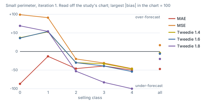
Figure 8. Bias by selling class for five of the objectives, scaled so the largest absolute bias in the chart is 100.
- The metric was fixed to be the same as the objective function. This allowed the early stopping to be even more effective in stopping additional iterations, and made the results more comparable.
- Using the log likelihood of the distribution of the target, we also calculated the theoretical optimal power variance to be 1.59. In practice, we tested multiple values and 1.5 seems to perform best.
- The objective function and metric have the most differentiating effect on the result.
Step 2: complexity of trees
- num_leaves: [512, 1024, 2048, 4096, 8192, …]
- min_data_in_leaf: [10, 50, 100, 300]
- 20 variations, to fix num_leaves and min_data_in_leaf
To choose the best combinations, we proceeded as follows:
- choosing the best min_data_in_leaf for each num_leaves: we found 50 and 300 are almost always the best
- choosing the best num_leaves for 50 and for 300
- 2 tendencies seem to dominate: small num_leaves with big min_data_in_leaf, and vice versa (512 leaves with 300, and 2048 leaves with 50)
- we choose to test the regularization for 2048 leaves with min_data_in_leaf 50
Step 3: regularization
- L1_regularization: [0, 0.2, 3, 0.8]
- L2_regularization: [0, 0.2, 3, 0.8]
- boosting: [‘gbdt’, ‘dart’]
- 9 variations
Note: these two regularization terms have different effects on the weights; L2 regularization (controlled by the lambda term) encourages the weights to be small, whereas L1 regularization (controlled by the alpha term) encourages sparsity, so it encourages weights to go to 0. In LightGBM the weights are the leaf values:
L = sum_i loss(y_i, h(x_i)) + 1/2 * lambda * sum_j w_j^2 + alpha * sum_j |w_j|The results of this first test will be used to derive general tendencies about which hyperparameters work best. We will test the ones that are most interesting on the full 3 perimeters scope. Results show that more regularization gives better results.
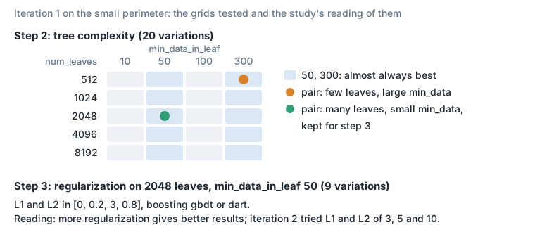
Figure 9. Iteration 1, steps 2 and 3: the grids and what the study kept from them.
Iteration 2: test on 3 perimeters
Step 1: objective function
- objective: [tweedie]
- tweedie_variance_power: [1.4, 1.5, 1.6]
- 3 variations, to fix the objective function
Results displayed are for the medium and small perimeters. Best: variance 1.6.
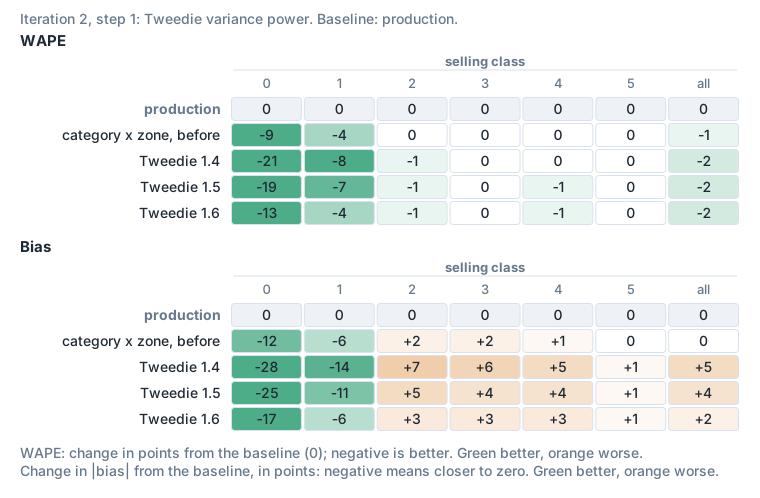
Figure 10. Iteration 2, step 1, relative to production.
Step 2: complexity of trees
- num_leaves: [64, 256, 512, 1024, 2048]
- min_data_in_leaf: [50, 300]
- 10 variations, to fix num_leaves and min_data_in_leaf
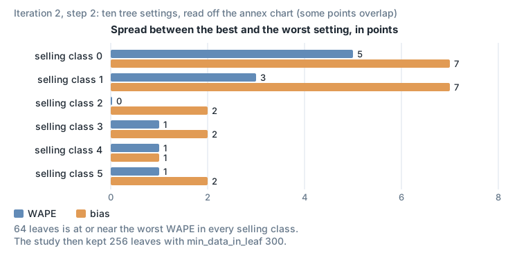
Figure 11. Iteration 2, step 2, from the study’s annex: how far apart the ten settings are, per selling class.
Step 3: regularization
- L1_regularization: [3, 5, 10]
- L2_regularization: [3, 5, 10]
- boosting: [‘gbdt’]
- 3 variations
Results displayed are for the medium and small perimeters. Best: L1 3 and L2 3.
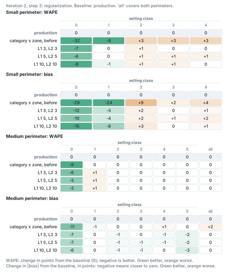
Figure 12. Iteration 2, step 3, relative to production.
Analysis
Objective function
Tweedie distribution with different power variances. Increasing the power variance shifts mass away from zero towards the right. For a power between 1 and 2, the Tweedie distribution has a point mass at zero and a continuous, right-skewed density on positive values (a compound Poisson gamma distribution, see scikit-learn’s generalized linear models).
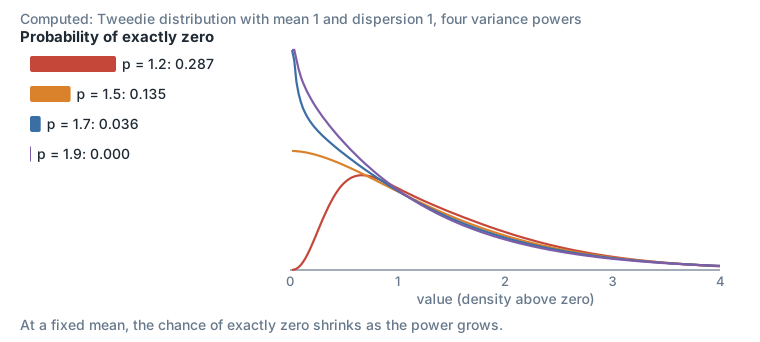
Figure 13. Computed, not from our data: a Tweedie distribution with mean 1 and dispersion 1 for four powers.
Theoretical analysis on the Tweedie power variance: we used negative log likelihood to fit a Tweedie function to the distribution of sales for each country in one product category. We also ran experiments with Tweedie 1.4, 1.5 and 1.6 and determined the optimal power variance. Below is a comparison of the optimal values, theoretical and experimental (WAPE + |Bias| as the metric):
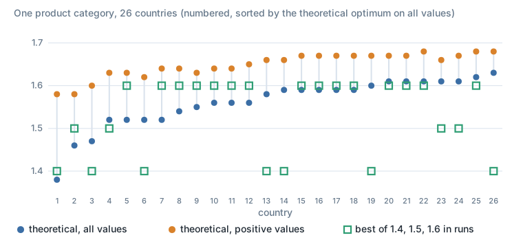
Figure 14. Optimal Tweedie variance power per country, from the fit and from the runs. Countries are numbered.
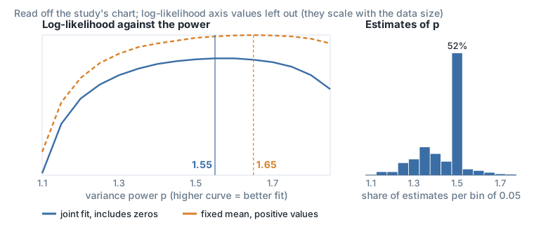
Figure 15. The fit behind the theoretical optimum: log-likelihood against the power for a joint fit including zeros (best at 1.55) and a fixed-mean fit on positive values (best at 1.65), and the distribution of power estimates.
We conclude that there is a correlation between the theoretical and experimental optimal power variance; in the future we can use the theoretical method to further optimize our power variance choices.
Optimizing for high sellers
The loss induced by each objective function incurred by missing the target by 1 sale:
- we can observe that for the Tweedie and gamma the loss is lower the higher the sale, which means the model is penalized more for low sellers misses than for high sellers ones
- MSE keeps the loss rate similar
- we can create a function that actually increases the loss the higher the sales, by multiplying the MSE error by y_target
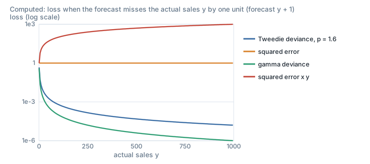
Figure 16. Computed from the loss formulas (Tweedie deviance), not from our data.
Gain in leaves distribution. We fixed min_gain_to_split = 0 so that the model adds additional splits in the trees even if the gain from those splits is very minimal. The distribution of the gain resulting from each split for a model shows that most splits add a gain lower than 100, with a peak around 2. However:
- it’s difficult to constrain min_gain_to_split because it depends on the individual case
- the gain of a split is proportional to the reduction in training loss that the split brings (a second-order estimate from the gradients and hessians). The loss using Tweedie, for example, is higher for lower sellers, so by restricting min_gain_to_split we are more likely to stop splits that would increase the performance on the high sellers as opposed to low sellers
In LightGBM, the gain of a split with L1 term alpha and L2 term lambda is:
split_gain = T(G_left)^2 / (H_left + lambda) + T(G_right)^2 / (H_right + lambda) - T(G_parent)^2 / (H_parent + lambda)
T(G) = sign(G) * max(0, |G| - alpha)
where G and H are the sums of the gradients and hessians of the rows in each node, and the parent term is thresholded by alpha too (source).
Sales distribution. The distribution of our training set is a determinant factor for the model: if it’s biased towards low sellers, the model will optimize more for low sellers. Our sales distribution is right skewed, but it’s moderately balanced due to the split groups calculation, when we filter most of the low sellers. Our training distribution is defined by items in:
- the top 3% of products by sales volume
- items that represent more than 5% of the sales of their group, defined by store x sub-department
- 2% randomly chosen items from the entire population
We can optimize more by reducing further the volume of low sellers, but overall our current method results in a pretty balanced distribution.
Sample weighting. We’ve established that using Tweedie we actually have more loss for misses on low sellers. This behaviour isn’t ideal; we want equivalent or even higher losses for higher sellers. To communicate this different processing to the model, we introduced sample weights where we give higher importance to high sellers samples. As a first approach we used log(target + 1) to define the importance of a sample.
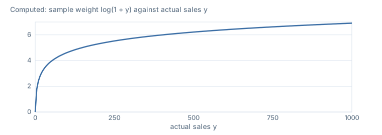
Figure 17. The weighting function, computed.
We ran the experiment on the medium and small perimeters:
- all methods except the reference (Tweedie 1.6 from iteration 2, step 1) used a sample weighting as defined above
- the difference between tweedie_mg0, tweedie_mg1 and tweedie_mg10 is only the value of the min gain to split hyperparameter
- the difference between tweedie_mg0 and tweedie_val_high is that tweedie_val_high limits the choice of validation set to only high sellers
- gamma uses the gamma objective and metric functions; it necessitates having a strictly positive dataset. We filtered our dataset in this sense before training
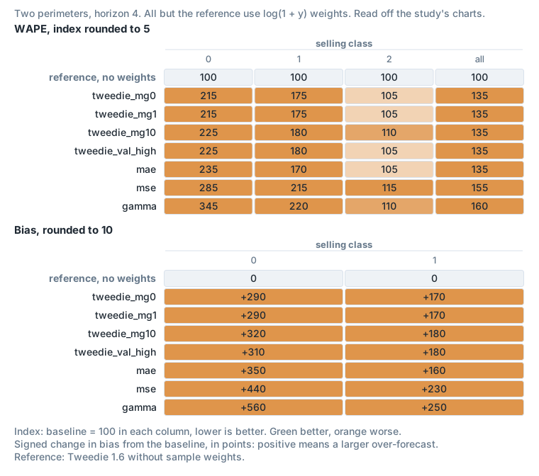
Figure 18. Sample weighting runs, relative to the unweighted Tweedie 1.6 reference.
The results show the following:
- Sample weighting
- efficiently gets the model to overforecast rather than underforecast; we no longer see the familiar trend of underforecasting high sellers.
- decreases the accuracy on low sellers, but without increasing it sufficiently on high sellers. Perhaps we weighed the low sellers too disadvantageously using the log function; we could experiment with a simpler weighting in the future (1 for low sellers, 2 or 3 for high sellers).
- min_gain_to_split
- increasing min gain to split decreases the accuracy on the low sellers, so it seems that it stops splits that would happen in the low sellers.
- there is a sweet spot of min gain to split = 1 which gives the best results; however getting this value right every time may be tricky.
- Objective functions
- Gamma is, as expected, very bad at low sellers since they aren’t a part of the training set. However this isn’t compensated by a better performance on the high sellers.
- MSE tends to overforecast a lot and often, in part due to sample weighting.
- MAE is close to the performance of the Tweedie and does present some potential, both in terms of WAPE and bias.
- Tweedie remains the best possible compromise between low sellers and high sellers.
Challenges with the experiment
- WAPE
- it is biased towards the low sellers (predicting 2 instead of 1 is a 100% error while predicting 200 instead of 199 is 0.5% error); however from a business value perspective, they should have almost the same effect.
- For trending data, WAPE doesn’t converge to a stable value. With a linear trend example, the WAPE is not a consistent estimator, because the denominator grows with the trend while the numerator (forecast errors) remains relatively stable.
- the weight w_t of an individual point of a low seller’s time series is higher than a similar point of a high seller:
WAPE = sum_t |y_t - y_hat_t| / sum_t |y_t|
= sum_t w_t * |y_t - y_hat_t| / |y_t|, with w_t = |y_t| / sum_t |y_t|- Looking at individual examples is time consuming and, unless there are major differences between the methods, doesn’t allow the selection of the optimal solution.
- We have more low sellers than we have high sellers, so most models naturally choose to overfit on low sellers patterns.
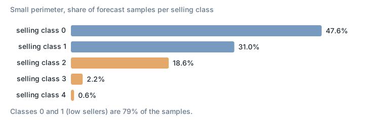
Figure 19. Forecast samples per selling class on the small perimeter, as shares.
- Even while using the Tweedie, models struggle to optimize for high and low sellers at the same time: we always overforecast low sellers and underforecast high sellers. It’s almost better to make 2 models, one for low and one for high sellers.
- Choosing the right objective function and metric is THE most important step in any optimization process.
- Adding our metric in the model training allows direct optimization, instead of optimizing RMSE or Tweedie and re-evaluating on WAPE.
Hyperparameters specialization
One of the big differences between the previous country cluster based modeling and the current product category x zone based modeling is the difference in sizes. In the product category x zone modeling we have many product categories with small amounts of rows. This necessitates hyperparameters that are different from those tuned on the larger clusters. Our three perimeters have about 20M (medium), 60M (large) and 0.9M (small) training rows.
From our training we also observe that the small clusters converge very quickly. They also require less complex trees than those of big clusters.
Training with the same set of hyperparameters for 3 types of clusters results in degraded performance. We therefore recommend splitting the clusters into 3 categories: big (> 40M rows), medium (between 1M and 40M) and small (< 1M), and using the following hyperparameters for each:
| Hyperparameter | Big cluster | Medium cluster | Small cluster |
|---|---|---|---|
| objective | tweedie | tweedie | tweedie |
| metric | tweedie | tweedie | tweedie |
| tweedie_variance_power | 1.6 | 1.6 | 1.6 |
| boosting | gbdt | gbdt | gbdt |
| bagging_freq | 1 | 1 | 1 |
| bagging_fraction | 0.9 | 0.8 | 0.7 |
| feature_fraction | 0.8 | 0.8 | 0.8 |
| learning_rate | 0.07 | 0.05 | 0.03 |
| max_depth | -1 | -1 | -1 |
| min_data_in_leaf | 300 | 300 | 300 |
| num_iterations | 3000 | 3000 | 3000 |
| num_leaves | 256 | 256 | 256 |
| lambda_l1 | 3 | 3 | 3 |
| lambda_l2 | 3 | 3 | 3 |
| min_gain_to_split | 0 | 0 | 0 |
- The larger the dataset, the larger min_data_in_leaf and num_leaves.
- The larger the dataset, the higher the learning_rate (to save time).
- Use a lower feature_fraction for smaller datasets to introduce more randomness and combat overfitting, which is a heightened risk in limited data (as LightGBM’s leaf-wise growth can lead to complex trees that memorize noise; the LightGBM documentation notes that leaf-wise growth may cause over-fitting when data is small).
Conclusion
| Hyperparameter | Old | New |
|---|---|---|
| objective | tweedie | tweedie |
| metric | rmse | tweedie |
| tweedie_variance_power | 1.6 | 1.6 |
| boosting | gbdt | gbdt |
| bagging_freq | 1 | 1 |
| bagging_fraction | 1 | 0.8 |
| feature_fraction | 0.8 | 0.8 |
| learning_rate | 0.07 | 0.05 |
| max_depth | 256 | -1 |
| min_data_in_leaf | 100 | 300 |
| num_iterations | 1000 | 3000 |
| num_leaves | 1024 | 256 |
| lambda_l1 | 0 | 3 |
| lambda_l2 | 0 | 3 |
| min_gain_to_split | 0 | 0 |
References
- Beginner’s guide to the must-know LightGBM hyperparameters
- L1 and L2 regularization in LightGBM
- What is elastic net regularization, and how does it solve the drawbacks of ridge and lasso?
- Master LightGBM efficiently to make predictions
- Gradient boosting and XGBoost
Feature Set Study
Summary of findings
This study aimed to determine the most effective feature set to support the change to our product category x zone modeling approach.
Our experimentations were conducted in a structured way and based on the results of the following analysis:
- Metrics: determined by WAPE and Bias. Our focus remains to optimize for high sellers (sc > 2).
- Visualizations: the examples were chosen to represent the best and worst results obtained by our current production model.
- Explainability:
- beeswarm plot: to determine the impact of each feature on the model
- bar cohorts plot: for categorical features, to determine how the impact of the features on the model varies for different cohorts of the categorical features
- feature correlation plot: uncovers the correlation between features given a clustering cutoff that represents the distance between features (0 = collinear features)
In the two steps of the experiments, we tested various feature sets. The goal was to remove features that don’t have any impact on the model and features that are strongly correlated.
We concluded the study by specifying one set of features which we deem the optimal one. The chosen feature set reflects our key conclusions:
- Having strongly correlated features in the model causes the latter to split ~randomly on either feature, which ends up hurting performance.
- Removing the most important sales derived features forces the model to derive new relations from the remaining features.
- Removing second order sales derived features (lag 2, the last-year lag and the average two months ago) actually improves the model, freeing up the model to use other features.
- Removing the most important sales derived features is detrimental to the model’s performance.
- Removing unnecessary features from the model speeds up training and inference time significantly.
For high sellers, our main focus, the chosen feature set allowed up to 3 points of WAPE improvement over the product category x zone baseline and up to 6 points of bias improvement over the product category x zone baseline.
Intro
The goal of this study is to determine which combination of features provides the best forecast performance, using hyperparameters from the hyperparameter set study.
Perimeter: the medium, large and small perimeters, each with its cutoff.
Across all experiments, multiple sets of features have been tested. Forecasts have been compared to those in production and those referring to the “product category x zone” split (actual hyperparameters and features). To find the best combination of features, metrics and visualisations have been computed, along with additional feature importance plots to assess the relevance of using some features.
Setup of the Experimentation
Terminology:
- Base features: the existing production model features
- New features: the newly introduced price, calendar and sku/bu features
- Sales derived features: all lags, baseline quantity and the average sales features
We structured the tests in two stages:
- First stage: 5 feature sets were defined and compared. The selection of features for these sets took into account both the feature category (sku/bu, holidays, price, lags) and the rankings obtained by analyzing the feature importances from the hyperparameter experiments.
- allfeatures: use every feature available in the preprocessing (new + base)
- minimalist: keep only the “most important” new features from feature explainability (per feature category below) + all base features
- minimalist_base: with respect to minimalist, removing second order sales derived features
- minimalist_inversebase: same as minimalist_base but keeping second order sales derived features and removing the rest
- minimalist_inversenew: with respect to minimalist, choose unselected new features for sku/bu, holidays and price features and remove the most important new features
- Second stage: the feature set that delivered the best results was then used as a baseline to construct 3 additional sets, including one that excluded sales lags. The objective here was to assess whether the final model could be improved by adjusting certain variables, based on insights from the first stage models.
- minimalist_split1: with respect to the minimalist_base set, keep global features for sku/bu, holidays and price
- minimalist_split2: with respect to the minimalist_base set, keep local features for sku/bu, holidays and price
- minimalist_withoutlag: with respect to the minimalist_base set, remove all sales derived features
The following table shows the list of feature sets and their composition.
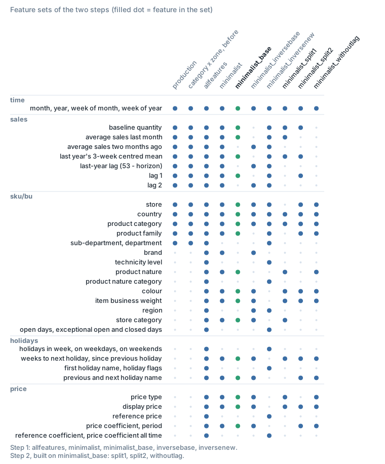
Figure 20. Feature sets and their composition.
Each of the tested models uses the set of hyperparameters defined during the hyperparameter experiments.
Detailed Results
Step 1: metrics
Results here are presented for the medium and small perimeters.
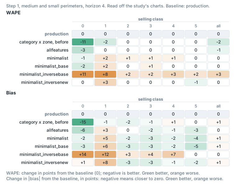
Figure 21. Step 1, relative to production.
We can observe that the “minimalist_base” model performs better in terms of bias while achieving a WAPE similar to the other models. Therefore, we selected it as the basis for further iterations and introduced some improvements in a second step.
Step 1: visualization
The examples were chosen to represent the best and worst results obtained by our current production model. They show single products’ weekly sales, so they are not reproduced here.
Step 1: explainability
The following represent the feature importance for the different sets of features on different perimeters. We can observe the following:
- Many features in inversenew don’t have any influence on the model, which confirms our initial choice of new features (inversenew has the inverse of what we deemed the most important new features).
- The order of importance of features existing in minimalist and minimalist_base remains the same (minimalist_base has the same features as minimalist, but with the removal of additional base features).
- The inversebase feature set was meant to test the effectiveness of removing the best performing base features. We can observe the use of newly introduced features more by the model (display price and brand, for example). This however didn’t replace the sales derived features’ added value.
- Using less influential sales derived features in inversebase forced the model to identify new ways to use the other features: we see that the importance of price and sku/bu features increased significantly. However, this is still not enough to replace the absence of the most influential sales derived features (baseline quantity, average sales last month and lag 1), which keep the model lagging behind performance wise.
Regarding some of the base features: we noticed that the behaviour of last year’s 3-week centred mean at horizon 1 is counterintuitive: when this feature is high, the model decreases its prediction. When looking closely, we discovered that this is due mainly to price type: when the latter is equal to “end of line”, last year’s 3-week centred mean happens to be high. The distribution of price type is clearly different for these rows, and price type is actually the feature that influences the model to decrease predictions.
Regarding price features:
- the importance of the different features is as follows: price type > display price > price coefficient for the period, price coefficient all time, reference price > reference coefficient
- “drop” doesn’t have as much impact as “end of line”
- display price has more importance when the price is missing, which makes sense
- the price coefficient for the period (display price / reference price) seems to have more impact than the price coefficient all time (display price / largest reference price of all time). This could be explained by the fact that customers aren’t aware of the past reference price, but only of the current reference price, so they base their purchase decision on that.
- we decide that the most important price features are:
- display price: shows the same distribution in cohort plots as reference price
- price coefficient for the period: shows the same distribution in cohort plots as the price coefficient all time
- price type: provides a unique distribution in cohort plots
From a performance point of view, minimalist_base was the most consistent method.
To choose the feature set for the second set of experiments, we looked at the correlation between features (the features that have a similarity of more than 70%). We can observe the following similar sets of features:
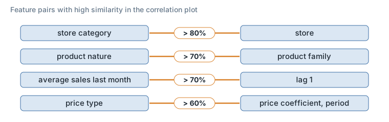
Figure 22. Similar feature pairs in the correlation plot.
We therefore decided to remove each of the features for one of the sets we tested in step 2 (split1 and split2).
Step 2: metrics
Results here are presented for the medium and small perimeters, by cutoff and selling class.
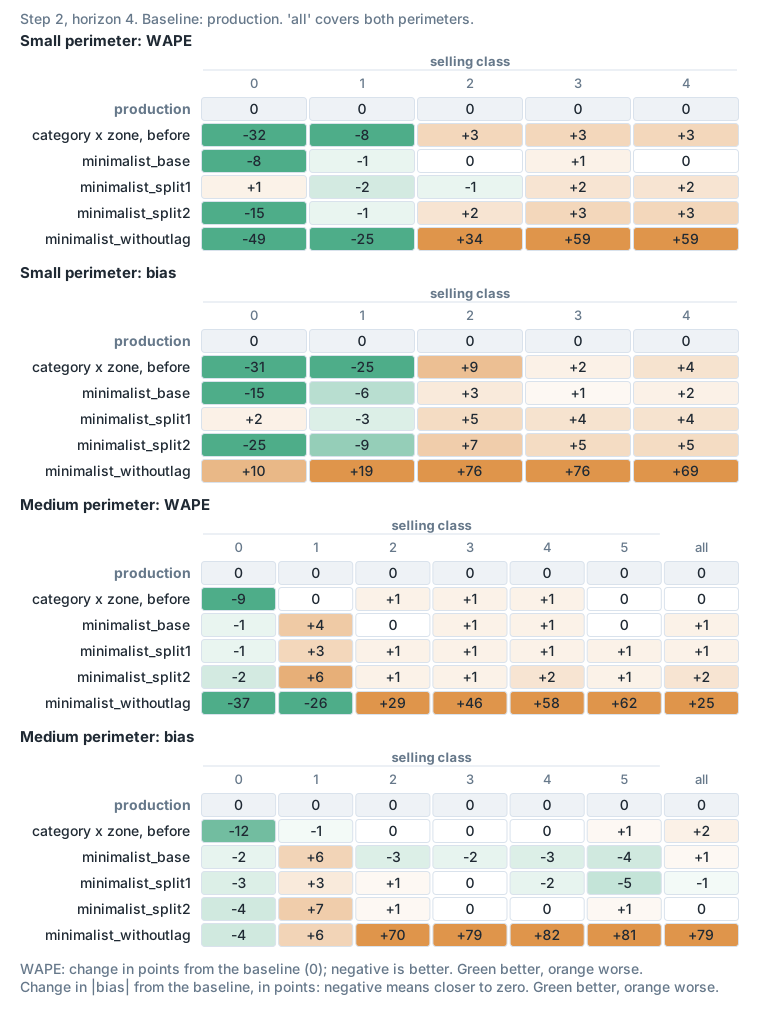
Figure 23. Step 2, relative to production.
With this second step, we observe that the “minimalist_base” model still stands out among the best. The variant without sales lags performs very poorly, most likely because the model is misled by the low-selling classes, which make up the majority of the data.
Step 2: visualization
The same comparison on single products, on the medium and small perimeters and then on the large one, is not reproduced here for the same reason.
Step 2: explainability
The following represent the feature importance for the different sets of features for different perimeters. We can observe that:
- When on their own, “store category” and “store” don’t impact the model as much as we would have hoped in split1 and split2. Actually store seems to be more important in minimalist_base, in the presence of store category.
- In the absence of sales derived features, store category and the number of weeks to the next holiday dominate the impact on the model.
- Comparing split1 to base: when removing features, the impact of the remaining features on the model increases (average sales last month and baseline quantity, for example).
- Comparing split2 to split1: the impact of sales derived features, which remain constant between the two sets, is drastically different. Split1 doubles down on sales derived features, while split2 actually uses new features more.
- Features in withoutlag have the least impact on the model per feature; this also explains the poor performance of this model: there simply isn’t enough information in those features.
- For the small perimeter, we observe that the number of weeks to the next holiday has a huge effect on the model.
Step 3: feature fraction
To combine the importance of deriving new relationships from less correlated features with the powerful effect of the sales derived features, we can use feature fraction to reduce the fraction of features used in each tree.
- in minimalist_base: feature fraction set to 0.8
- in the first variant: feature fraction set to 0.6
- in the second variant: feature fraction set to 0.4
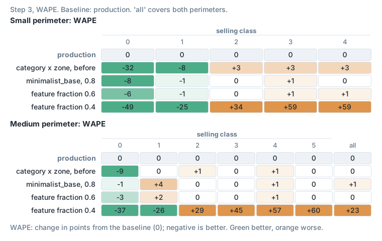
Figure 24. Feature fraction, relative to production.
Feature fraction set to 0.4 seems to be too low, so that it drastically reduces the performance of the model. 0.6 is very close to 0.8, which remains the optimal value.
Conclusion
We conclude the study by keeping minimalist_base as our most optimal feature set. We base our decision on the following:
- Having strongly correlated features in the model causes the latter to split ~randomly on either feature, which ends up hurting performance.
- Removing the most important sales derived features forces the model to derive new relations from the remaining features.
- Removing second order sales derived features (lag 2, the last-year lag and the average two months ago) actually improves the model, freeing up the model to use other features.
- Removing the most important sales derived features is detrimental to the model’s performance.
- Removing unnecessary features from the model speeds up training and inference time significantly.
- Feature fraction can help the model get the benefits of deriving new relationships from less dominant features while using the dominant features in the model.
For high sellers, our main focus, the chosen feature set allowed up to 3 points of WAPE improvement over the product category x zone baseline and up to 6 points of bias improvement over the product category x zone baseline. This improvement will be validated by the backtesting, where we’ll test the feature set on a multitude of perimeters and cutoffs.
Compared to the production model, the switch to the product category x zone strategy suffered from a degradation of WAPE and bias for small perimeters, while improving performance on big perimeters (not shown here). With our chosen feature set, we’ve removed the negative effect on small perimeters while keeping the positive effect on big perimeters. We’ve even improved the bias over the production model in some cases.
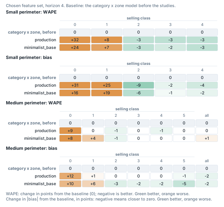
Figure 25. The chosen feature set, relative to the product category x zone model before the studies.
Future improvements
- Removing product category from the feature set, as it doesn’t vary within a product category x zone model.
- Many missing values appear in the features that we added (price type, next holiday name, colour, …). It’s worth investigating and fixing the source data if it’s an issue. Some could be justified, such as products with mixed colours.
- The price features were implemented to correspond to the forecasted week or to correspond to the prediction week; the latter, although functional, was more complicated in the preprocessing, so it was decided to save it for a future improvement. This should definitely improve the efficacy of the price feature.
- The same holidays have different names in different countries in some instances (for example one holiday under its local-language name in one country and under two different English names in others). This isn’t handled but should be handled in the preprocessing, to unite the same holidays under the same name.
Annex: metrics with variations of minimalist_base on all perimeters
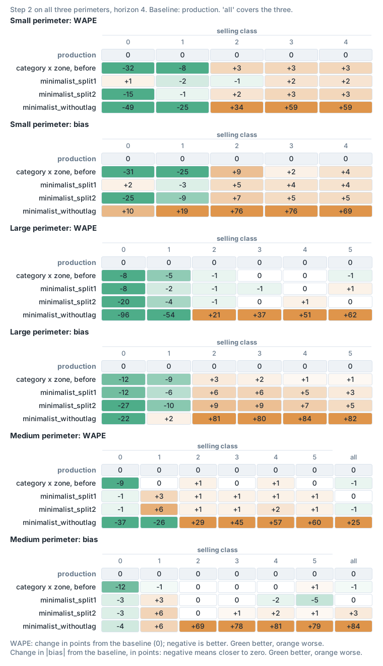
Figure 26. The step 2 sets on all three perimeters, including the large one, relative to production.