Tabular foundation models
Tabular foundation models (TFMs) are pretrained networks that predict on a table they have never seen. The best known are TabPFN (PFN for prior-data fitted network, by Prior Labs), TabICL (ICL for in-context learning, by the SODA team at Inria) and Google’s TabFM. This post explains how they predict; the companion post tests them on a real sales forecast.
With LightGBM, fit() is where the work happens: the model looks at your rows and builds trees. With a TFM, fit() mostly stores your table (plus light preprocessing, and optionally a cache; see How the cost grows). The work happens in predict(): the stored rows (the context) and the rows you want answered (the test rows) go through the network together in one forward pass (in practice a few passes on shuffled copies of the table, averaged; see How the cost grows). The weights never change. This is called in-context learning: no training on your data.
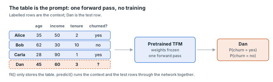
The labelled rows are the context; Dan is the test row.
The running example
One small churn table is used all the way through: three customers have a known answer, and we predict the fourth.
| Customer | age | income (k€) | tenure (years) | churned? |
|---|---|---|---|---|
| Alice | 35 | 50 | 2 | yes |
| Bob | 62 | 30 | 10 | no |
| Carla | 28 | 90 | 1 | yes |
| Dan | 45 | 60 | 3 | ? |
- n = number of rows = 4: three labelled rows, the context (Alice, Bob, Carla), and one test row to predict (Dan). We write n_ctx = 3 and n_test = 1 for their counts.
- d = number of feature columns = 3 (age, income, tenure). The label column, churned?, is not counted in d.
- A cell = one value at one row and one column. Example: Alice’s age is the cell 35.
- A vector = a list of numbers. Example: [0.1, −0.4, 0.7].
- e = the length of each cell’s vector: 128 in TabICL (a row in stage 3 is 4e = 512).
Real tables have thousands of rows and dozens of columns. The steps are exactly the same.
The model described is TabICL v1, from the 2025 paper. The current tabicl package ships TabICLv2; its main changes are listed after the three stages. Sizes such as 128 are TabICL’s; other models use other sizes.
How it predicts: three stages
The big picture
A transformer works on tokens, the units it compares with each other. For text, a token is a piece of a word. For a table, there are three choices:
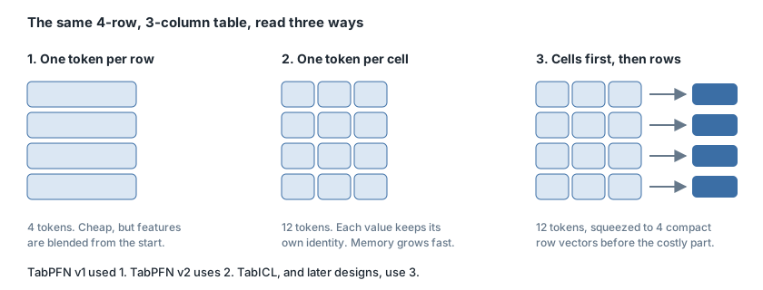
TabPFN v2, the cell-per-token design here, actually puts two cells of a row in each token by default.
One token per cell keeps each value’s identity, but the number of tokens is rows times columns, so it is expensive. The newer designs start with cells and then compress each row into one vector before the step where rows are compared with each other, the expensive one.
TabICL is one of those newer designs. It runs the same kind of transformer block in three stages; each stage lets a different set of things look at each other.

TabICL-style pipeline, with the shapes for the example table
Stage 1 turns each number into a vector, stage 2 turns each row into one vector, and stage 3 lets Dan’s row read the labelled rows to predict his answer. Each stage answers one question:
- Stage 1: where does this cell sit in its column’s distribution?
- Stage 2: taking all of this row’s values together, what kind of row is this?
- Stage 3: which labelled rows resemble this one, and what were their answers?
- Head: so what is the probability of each class?
Attention in one picture
Every stage uses the same block (stage 1 runs it through inducing points, below). Only two things change: what one token is (a cell, then a row) and who may look at whom.
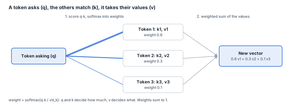
One attention step. d_k is the length of one head’s slice, defined below.
Each token carries three vectors, made by multiplying it with three learned matrices, W_Q, W_K and W_V:
- the query q: what this token is looking for;
- the key k: what this token offers to others;
- the value v: what this token passes on if it is chosen.
Each of these vectors has the length of the token itself, e = 128 numbers in stages 1 and 2, 4e = 512 in stage 3. The block splits them into several slices, called heads, and runs the same attention on each slice side by side; d_k is the length of one slice. The heads’ outputs are glued back together and projected to the token’s length.
In each head, the token asking takes the dot product of its q with the k of every token it is allowed to look at. Each dot product is a single number, a score. A softmax turns the scores into weights that sum to 1, weight = softmax(q·k/√d_k). The token’s new vector is the weighted sum of the values: in the picture, 0.6 v1 + 0.3 v2 + 0.1 v3. q and k decide how much, v decides what.
After the attention, a small feed-forward network (FFN) runs on every token. Each of the two steps normalises its input, applies the step, and adds the result back to the input (a residual connection).
Stage 1: attention on the columns
Each cell becomes a vector that knows its column. 35 alone means nothing; 35 among ages 28 to 62 means “on the young side”. Stage 1 encodes that.
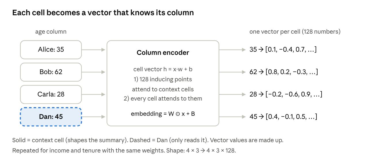
Stage 1 on the age column
It works on one column at a time, with the same weights for every column:
- Each number becomes a vector, h = x·w + b, with w and b learned: x is one number, h is that number as a vector of length e.
- A Set Transformer (a transformer that treats the column as an unordered set) reads the column. Letting every cell attend to every other cell would cost rows², so it uses m = 128 inducing points instead: a fixed set of learned vectors that first read the context cells of the column, then are read by every cell. Cost grows linearly with rows instead of quadratically. TabICL stacks 3 of these blocks.
- The Set Transformer outputs, for each cell, a weight vector W and a bias vector B. The cell’s embedding is W ⊙ x + B (each of W’s 128 numbers multiplied by x, plus B): the raw number again, scaled and shifted by what the column looks like.
Like a normalisation, this makes values comparable across columns, but it is learned, and the output is 128 numbers per cell instead of one. In practice, you don’t have to scale your columns: stage 1 does it. Only context cells shape the summary: Dan’s cell reads it but does not write to it. That is the first, small way a test row uses the context rows.
Stage 2: attention on the rows
Stage 3 compares rows, so every row must become one vector of the same size, whether the table has 3 columns or 600.
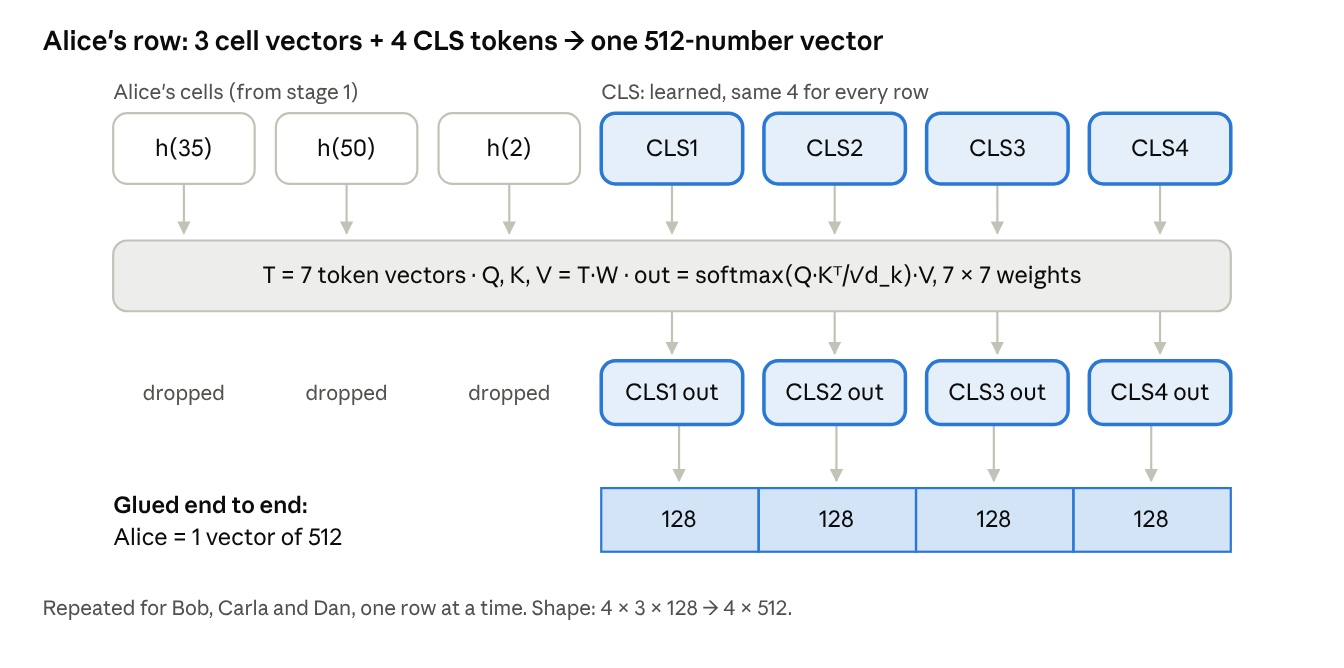
Stage 2 on Alice’s row. Here h(35) means Alice’s age after all of stage 1 (its W ⊙ x + B embedding), not the x·w + b vector of step 1; W in the box stands for the attention matrices W_Q, W_K, W_V.
Stage 2 is a 3-layer transformer that runs on each row separately. Its tokens are the row’s cell vectors plus 4 CLS tokens (CLS for classification token, a name from BERT).
- The CLS tokens are not data: they are 4 vectors learned in pretraining, the same 4 starting vectors for every row of every table, like blank notebooks each row fills in with its own summary.
- Stage 2 outputs the 4 CLS vectors of 128 numbers, then glues them end to end into 1 vector of 4 × 128 = 512. Toy version: [0.2, 0.5], [0.9, 0.0], [−0.4, 0.1] and [0.7, −0.2] glued end to end give [0.2, 0.5, 0.9, 0.0, −0.4, 0.1, 0.7, −0.2].
- Attention stays inside each row: stage 2 mixes nothing between rows.
- Column order matters here. Stage 2 rotates each query and key by an angle set by its column position (rotary positions), so moving a column changes the attention scores. In practice you don’t have to worry about it: the default ensemble shuffles the columns and averages.
Stage 3: in-context attention
Dan learns from the labelled rows. Now each token is a whole row, the 512-number vector from stage 2. Labelled rows get their answer added as a learned vector (one-hot class × a learned matrix); Dan asks, they answer. Stage 3 is a 12-layer transformer, the deepest of the three.
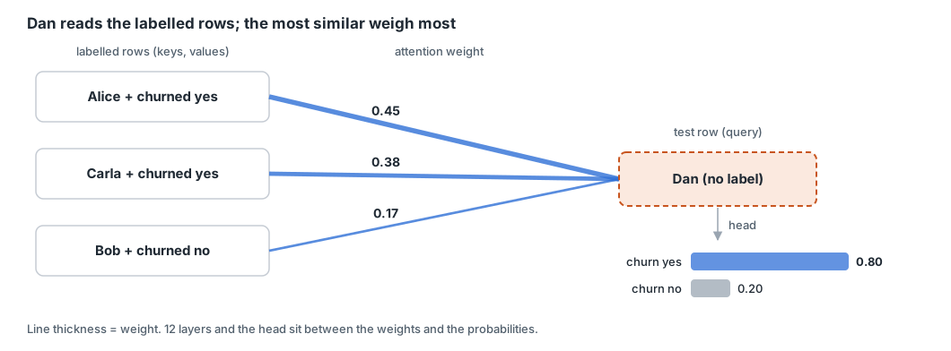
Stage 3: Dan attends to the labelled rows. Alice is closest to Dan on every column, and Carla is closer than Bob on tenure, so here they weigh most. In the real model, 12 layers of this and the MLP head produce the probabilities; they are not a sum of weights.
- No weights change: the learning happens inside one forward pass.
- This is where the test row mainly uses the context: it reads the labelled rows. Labelled rows also read each other in every layer, which is where the n_ctx² cost comes from, but they never read a test row.
- Test rows never attend to each other. Production rows often arrive one at a time, and keeping test rows apart makes each score independent of who else was in the batch.
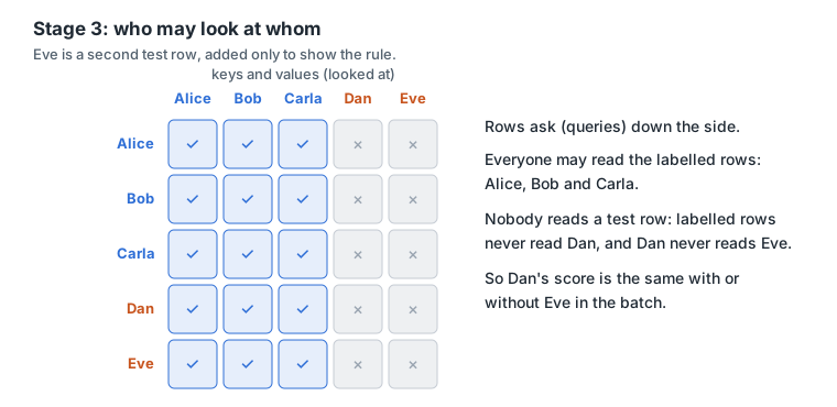
Who looks at whom in stage 3
Then the head turns Dan’s final vector into probabilities:
- Shape: Dan’s 1 × 512 → 1 × 2 (one test row, two classes). The head is a 2-layer MLP; TabICL v1 handles up to 10 classes natively, more through a hierarchy of classifiers.
- Class order matters here. Labels enter as one-hot vectors and leave through one output column per class, so changing which class gets index 0, 1, … changes which learned vectors are used. This is why TabICL’s default ensemble shifts the classes (and shuffles the columns, for stage 2’s rotary positions), then averages.
- TabICL v1 is classification-only; regression comes with TabICLv2, below.
Shapes at each step
The table shrinks from one number per cell to one probability per class for each test row.
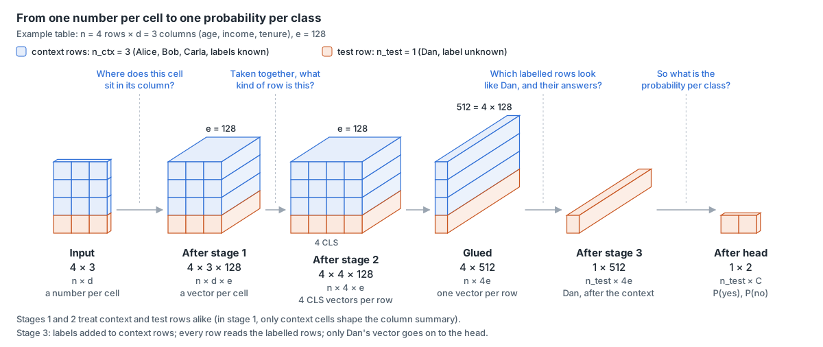
Tensor shapes for the example table, drawn AlexNet-style
C = number of classes. In the example, 4e = 4 × 128 = 512, so n × 4e in the table is the 4 × 512 above.
| Step | One token is | Attention runs | Our example | General |
|---|---|---|---|---|
| Input | none | nowhere | 4 × 3 | n × d |
| Stage 1 | one cell | down each column | 4 × 3 × 128 | n × d × e |
| Stage 2 | one cell or one CLS token | across each row | 4 × 7 × 128 in, CLS out 4 × 4 × 128, glued → 4 × 512 | n × (d + 4) × e → n × 4e |
| Stage 3 | one row | across rows: every row reads the labelled rows, never a test row | 4 × 512 in, Dan’s 1 × 512 kept | n × 4e in, n_test × 4e kept |
| Head | none | nowhere (an MLP on each test row) | 1 × 2 | n_test × C |
What TabICLv2 changes, and regression
TabICLv2 keeps the three stages, with three main changes: stage 1 embeds each cell together with two other cells of its row; the labels also come in at stage 1, not only at stage 3, so every stage knows the task; and each query is rescaled according to the context length and the query itself (QASSMax, query-aware scalable softmax), in stage 1’s inducing points and in stage 3.
It also adds regression, which changes only the head and the label vector. TabICLv2 predicts 999 quantiles, trained with the pinball loss used to score quantile forecasts, and its label goes in as y·w + b instead of a one-hot class vector. TabPFN does it differently: it cuts the range of targets into bins and outputs a probability per bin, a histogram with two thin tails, so training is a classification over bins and values beyond the outermost bins can only come from the tails. Either way, every prediction comes with a full distribution, so quantiles come for free.
How the cost grows
Stage 3 is the expensive one as the context grows: its attention grows with the square of the labelled rows, and linearly with the test rows. More columns never touch stage 3, because stage 2 has already squeezed each row into one vector.
With n_ctx, n_test, d and e as above, and m = 128 inducing points: attention-score cost = number of query-key pairs × the vector size of each dot product.
| Stage | Attention-score cost per layer | Rows | Columns |
|---|---|---|---|
| Stage 1, with inducing points (TabICL), per block | (2·n_ctx + n_test) × d × m × e | linear | linear |
| Stage 1, hypothetical without inducing points (not what TabICL does) | d × (n_ctx + n_test) × n_ctx × e | quadratic in n_ctx, linear in n_test | linear |
| Stage 2 | (n_ctx + n_test) × (d + 4)² × e | linear | quadratic |
| Stage 3 | (n_ctx² + n_test × n_ctx) × 4e | quadratic in n_ctx, linear in n_test | none |
Attention is not the whole bill. Every layer also projects each token into q, k and v, projects the result back, and runs an FFN: about 8 × width² multiply-adds per token, with width 128 in stages 1 and 2 and 512 in stage 3. And the stages have different depths: 3 inducing-point blocks, 3 row layers, 12 in-context layers. The two charts count all of it.
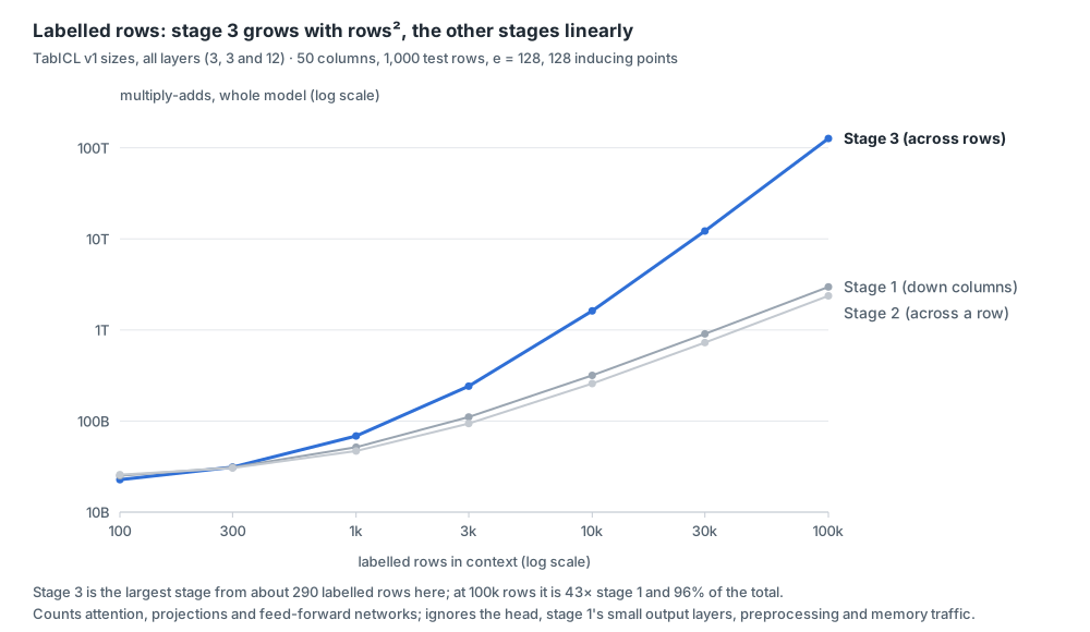
Computed by scripts/generate-tfm-prequel-figures.mjs from TabICL v1 sizes; the other sizes are in the subtitle
With 50 columns and 1,000 test rows, stage 3 is the largest stage from about 290 labelled rows, because it is the widest and the deepest. Past a few thousand rows its rows² term takes over: at 100,000 labelled rows it does 96% of the work.
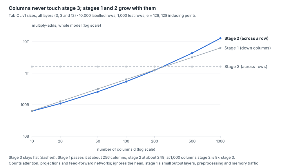
Computed by scripts/generate-tfm-prequel-figures.mjs from TabICL v1 sizes; the other sizes are in the subtitle
With 10,000 labelled rows fixed, stage 3 stays flat as columns grow (dashed line). Stages 1 and 2 both grow with the columns and pass stage 3 at about 250. Stage 2’s columns² attention only dominates its own cost past about 500 columns, so on very wide tables stage 2 pulls ahead of stage 1.
What doubling each input does to the attention-score cost (approximately; the projections and FFNs grow only linearly, so stage 2’s total is still about ×3 when doubling from 500 columns, and nears ×4 only on far wider tables):
| Double the… | Stage 1 | Stage 2 | Stage 3 | Overall |
|---|---|---|---|---|
| labelled rows (context) | ×2 when context rows dominate | ×2 when context rows dominate | ×4 when context rows dominate | ×4 once context is large |
| test rows | ×1 to ×2 | ×1 to ×2 | ×1 to ×2: only the test × context part doubles | at most ×2, close to ×1 when context rows dominate |
| columns | ×2 | ×4 for wide tables | ×1 | ×2 to ×4, stage 3 unaffected |
| vector size e | ×2 | ×2 | ×2 | ×2 in attention, ×4 in the projections and FFNs |
- Memory follows the same shape: stage 3’s attention-weight matrix has n × n_ctx entries per head and layer, unless the attention is computed in tiles (FlashAttention-style kernels).
- In practice, when the context is too large, subsample the labelled rows, retrieve the rows most similar to each test row, split the context and average (ensemble), or use a different model.
In practice, labelled rows never look at test rows, so their vectors can be computed once and reused (a KV cache; kv_cache=True in TabICL). Each new test row then pays stages 1 and 2 for its own cells and, in stage 3, about n_ctx × 4e per layer for attention plus its own projections and FFN, and test rows can be scored in parallel. Ensembling goes the other way: with n_estimators, the same frozen model runs on several views of the data and the predictions are averaged, so the default 8 estimators cost about 8 times one pass.
Training
Everything learned (all three stages, the CLS tokens, the label vectors and the head) was fixed during pretraining, before your data ever arrives.
The data is synthetic: tables nobody collected. Most come from a structural causal model, a random graph of causes and effects where some variables drive others and noise is added. The generator is highly parametrised, so it simulates simple and complex causal relationships alike. Sampling from one graph gives a small table, with one column as the target. In about 30% of TabICL’s tables, the cause-to-effect functions are tree models (XGBoost) instead of small neural networks, and TabPFN’s prior adds uninformative features, so the model learns to ignore them. The scale is large: about 130 million tables for TabPFN v2, about 83 million for TabICL, about 35 million for TabICLv2.
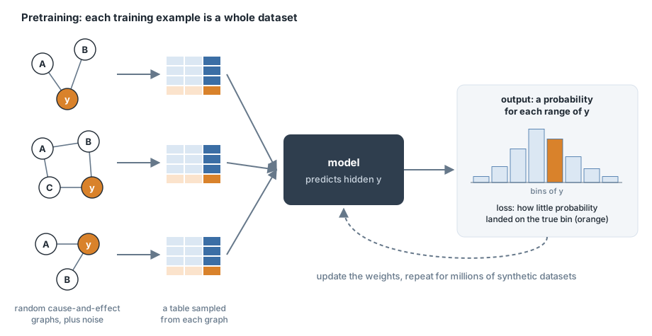
Shown for TabPFN-style regression, where the outputs are bins of y; for classification the bins are the classes.
The task is exactly the prediction setup: in each synthetic table, some rows are labelled and the rest are held out, and the model must predict the held-out labels. So each training example is a whole dataset, not a row. For classification the loss is cross-entropy: how little probability the model put on the true class. Tables usually grow during training (a curriculum): TabICLv2 trains on tables of 1,024 rows, then 400 to 10,240, then up to 60,000. What the model learns is a general skill, “given labelled rows, predict new rows”, rather than facts about any one dataset.
One caveat from training only on synthetic data: the model has never seen a real retail table. Promotions, sudden shocks and changes of regime are covered only as far as the generator produced something like them.
An LLM goes through pretraining, instruction fine-tuning, preference tuning (RLHF or DPO) and often RL for reasoning. A TFM is essentially one stage: pretraining on synthetic tables. Optional extras are continued training on real tables or fine-tuning on one client’s data. There is no preference tuning: the label already scores the prediction. The prior (the synthetic-data generator) does the job that data curation and alignment do for an LLM.
Why it works: prior-data fitted networks
TFMs are based on PFNs. A PFN approximates Bayesian model averaging. An example: a new product sold 0, 0, 5, 0, 0 and 6 units in its first six weeks. Is it bike-like (lumpy demand, most weeks zero) or sock-like (steady sales)? Say bike-like predicts 1 unit next week (most likely a zero week, with some chance of a spike) and sock-like 2 (its steady average).
You do not have to pick one. Score how well each explanation fits what you saw, turn the scores into weights, and average the two forecasts (both start equally likely):
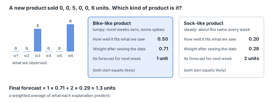
That is Bayesian model averaging. In symbols, with D the context (the labelled rows; not d, the column count), x the new row and φ one candidate task (one data-generating rule, such as one causal graph with its parameters): p(y | x, D) = ∫ p(y | x, φ) p(φ | D) dφ. For each candidate task, take its prediction at the new row, then weight it by how credible that task became after seeing the context.
The equation is exact under two assumptions: once you know the true task, the context tells you nothing more about the new answer; and the new row’s features, on their own, do not change which task is likely.
Doing this by hand means listing every possible task, which is impossible for real tables. A PFN learns to do it: trained on millions of tables from the synthetic generator, one forward pass approximates the average over every task that generator could produce. The generator is the “prior” in the name.
Comparison with the traditional transformer architecture
With “Attention Is All You Need”
Both use the same block: multi-head attention, then a feed-forward network (FFN), each with a residual connection and normalisation. What differs is how the blocks are wired and what a token is.
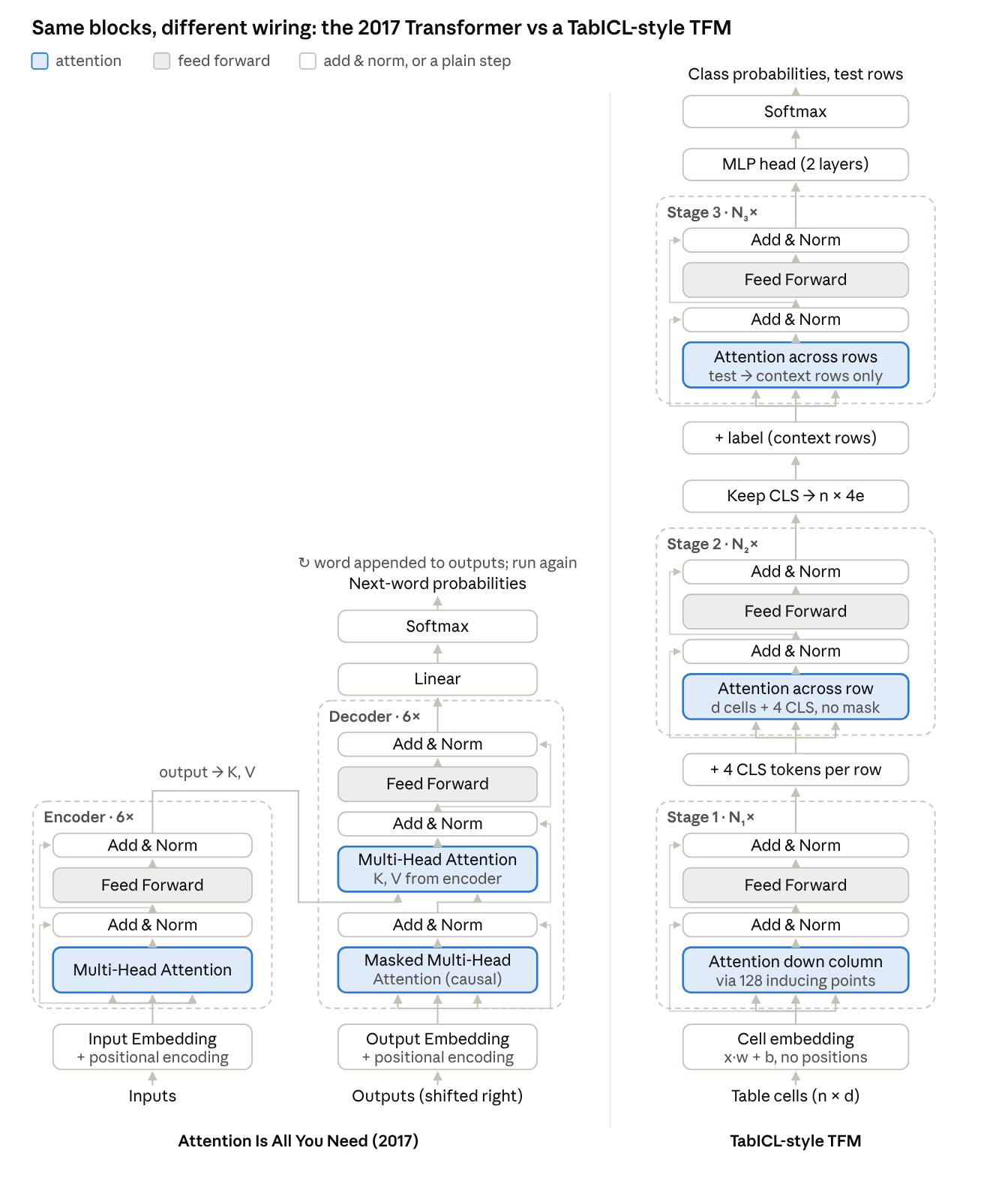
Original transformer vs TabICL-style TFM. In stage 3, context rows also attend to each other, not only test rows to context rows. Drawn with the 2017 paper’s Add & Norm after each step. Stage 1 outputs W ⊙ x + B, not just x·w + b. In TabICL v1, N₁ = 3 inducing-point blocks (each two attentions: points read cells, then cells read points), N₂ = 3 layers and N₃ = 12 layers.
The wiring differs: no decoder and no output fed back in; three encoder stacks run once, each along a different axis. The cross-attention that remains is inside those stacks (see the table), not from a decoder to an encoder. One detail differs too: the 2017 model normalises after each step, TabICL before it.
| Part | Attention Is All You Need (2017) | TabICL-style TFM |
|---|---|---|
| Task | translate a sentence | predict the labels of test rows |
| Family | encoder + decoder | encoder-style: no causal mask, one pass |
| One token | a word piece | a cell (stages 1 and 2), then a row (stage 3) |
| Embedding | a lookup table: one learned vector per word | x·w + b: a number times a learned vector |
| Position signal | on every token (word order matters) | none across rows (row order doesn’t matter); rotary positions across columns in stage 2 |
| Block | multi-head attention + FFN, add & norm | the same block |
| Stacks | encoder, then decoder | three stacks, one per axis |
| Masks | decoder: causal (a word sees only earlier words) | stage 1: inducing points read labelled cells only; stage 3: every row reads labelled rows only, never a test row |
| Cross-attention | decoder attends to the encoder’s output | stage 3: test rows (as queries) read labelled rows (as keys and values); also stage 1: inducing points read context cells |
| Output | one word per pass, repeated until the sentence ends | all class probabilities in one pass |
Since rows carry no position, the model has no idea which row is older: for time series, time has to be given as features (week of year, month, and so on).
With a modern LLM
Both are transformers that learn in context. They differ in what they were trained on, what a token is, and how they produce output. In practice an LLM is often the interface and orchestrator, and the TFM the prediction engine it calls.
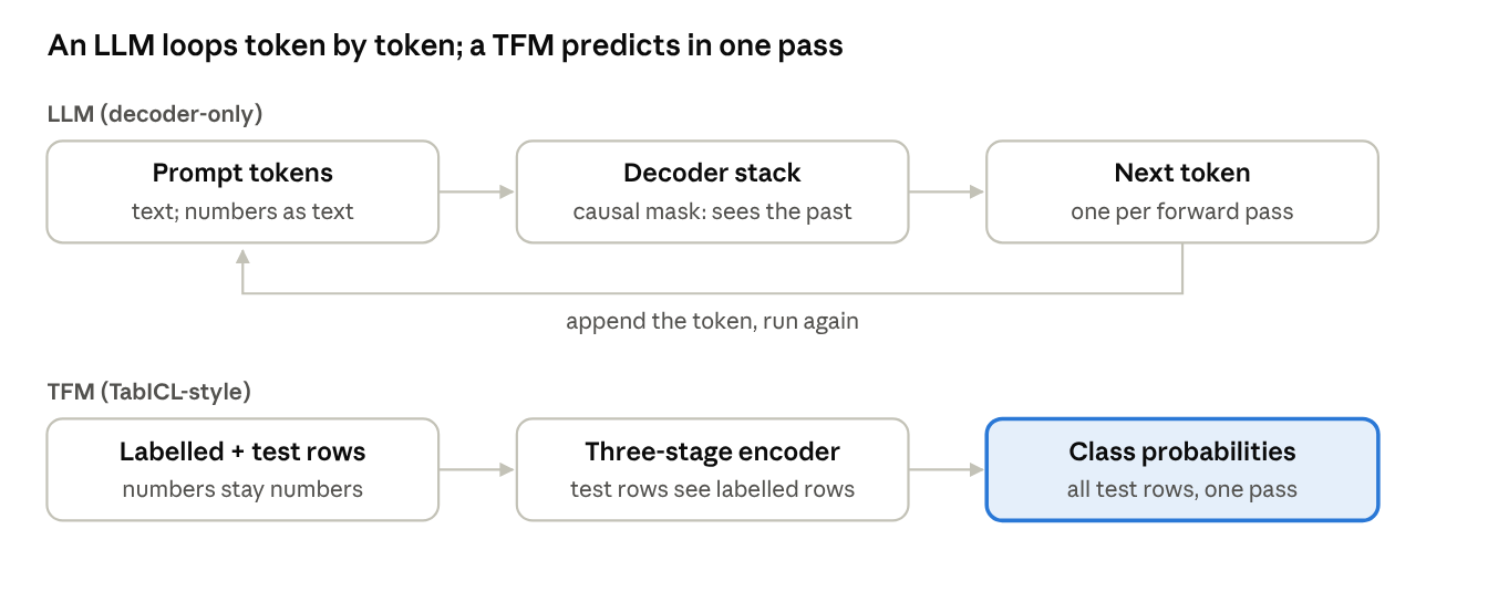
LLM vs TFM: loop vs one pass
| LLM | TabICL-style TFM | |
|---|---|---|
| Pretraining data | internet text and code | millions of synthetic tables from random causal models and tree-based generators |
| Pretraining task | predict the next token | predict held-out labels from labelled rows |
| What it learns | language and world knowledge | how to predict from examples |
| Input | a sequence; order matters | a table; row order doesn’t matter |
| Numbers | split into text tokens | fed in as numbers (x·w + b) |
| Wiring | decoder-only, causal mask | three attention stages; in stage 3 every row reads only labelled rows |
| Output | one token per pass, repeated | all predictions in one pass |
| Forecasting a horizon | step by step, each output fed back in | each future date is a test row; the whole horizon in one pass |
| In-context examples | written into the prompt | the labelled rows |
| Typical size | billions of parameters | typically a few million to tens of millions (TabPFN v2 ≈ 7M, TabICL ≈ 27 million; newest up to ≈ 215M) |
TabPFN-TS (TabPFN applied to time series, with calendar features as columns) forecasts this way, with no lags. A TFM forecast becomes recursive only with lag features shorter than the horizon. Time-series foundation models differ here: the original Chronos and Lag-Llama are autoregressive by design, while Chronos-Bolt and TimesFM predict a chunk of steps per pass and loop beyond it.
Other tabular foundation models: TabPFN and Kumo
This post follows the TabICL design; other tabular foundation models organise the same ideas differently.
TabPFN v2 and TabPFN-3
TabPFN v2 is a 12-layer transformer that never squeezes a row into one vector. Every cell is a token (in practice a pair of cells; see the token figure), and each of the 12 layers looks at the table in two directions. Down a column, a value is compared with the other values of the same feature: this is how the model knows whether 3.2 is high or low (like Dan’s age of 45 against 28 to 62). Across a row, the values of one example are combined.
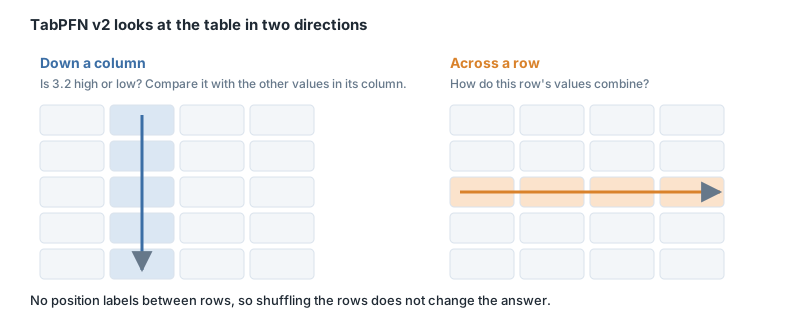
The catch is cost: every layer pays for rows² on every column. TabICL’s expensive in-context stage sees one vector per row instead of one per cell, which is what lets it take far more context rows. TabPFN-3 moved to the same column-then-row design: inducing-point column embedding, row compression with 4 CLS tokens, then 24 in-context layers; its report says the architecture is adapted from TabICLv2.
Kumo
Kumo, the start-up whose purchase by NVIDIA Fortune reported in June 2026, has two different models. Kumo Tabular (open weights, Sep 2026) works on one table and combines the two designs: TabPFN v2’s alternating column and row attention, then this post’s row compression and in-context stage. KumoRFM-2 (Apr 2026) works on a whole relational database and adds a stage that passes information between tables instead of flattening them.
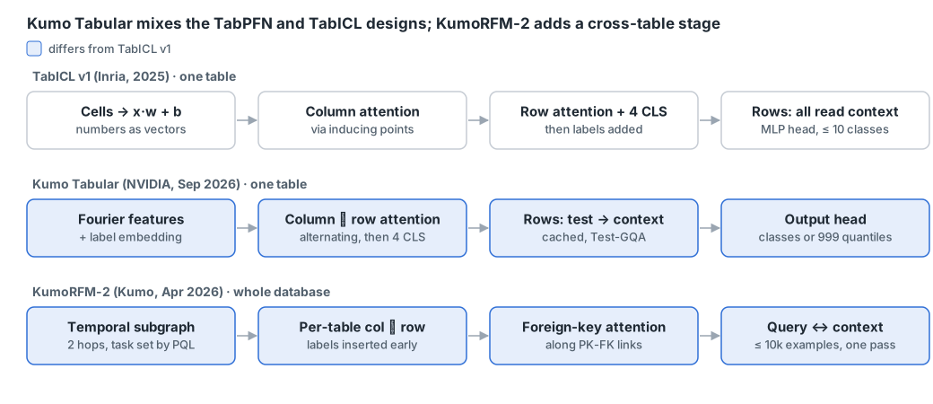
From NVIDIA’s Kumo Tabular blog and the KumoRFM / KumoRFM-2 papers, as of Nov 2026
| TabICL v1 | Kumo Tabular | KumoRFM-2 | |
|---|---|---|---|
| Input | one table | one table | a database as a temporal graph: records = nodes, primary key to foreign key (PK-FK) links = edges |
| Cell encoding | x·w + b, then W ⊙ x + B | Fourier features (learned sines and cosines); missing values handled natively | lightweight per-table encoder (few details published) |
| Who builds the labels | you supply X and y | you supply X and y | PQL (Kumo’s predictive query language) computes them at past timestamps, avoiding leakage |
| Output | MLP head, 10 classes per pass (more via a hierarchy) | ≤ 10 classes per pass (more via error-correcting codes); regression = 999 quantiles | classification, regression, multi-class, recommendation |
| Pretraining | synthetic (causal + tree priors) | synthetic only; 35M / 71M / 137M tables by size; curriculum: 1,024 rows, then 400 to 10,240, then up to 60,000 | synthetic + public real relational databases; single tables first, then relational |
| Size | ≈ 27 million parameters | 28M to 215M (3 sizes) | not stated |
| License | open (BSD) | OpenMDW-1.1, commercial use allowed | commercial product |
What Kumo changes:
- Kumo Tabular mixes the two families. It alternates column and row attention like TabPFN v2, then compresses each row with CLS tokens like TabICL.
- Labels enter early in both Kumo models (and in TabICLv2), so even the cell and row stages know what the task is. In TabICL v1 they only appear in stage 3.
- Built for scale: Test-GQA (a grouped-query attention variant for test rows), which the blog says shrinks the cache every prediction reads, and a length-aware temperature (it grows with the log of the number of keys) that keeps attention sharp on big tables.
- KumoRFM-2 refuses to flatten. Foreign-key attention lets an order pass information to its customer and products directly, and PQL builds point-in-time-correct labels.
Limits as published: Kumo Tabular was trained on up to 60,000 rows and 100 columns of context, and takes numerical and categorical columns natively; text, images and timestamps go through built-in preprocessing recipes. All benchmark results are self-reported: Kumo Tabular claims #1 on TabArena (Elo 1950); KumoRFM-2 claims up to 8% over baselines on relational benchmarks.
Much of Kumo Tabular’s recipe is also in the TabICLv2 paper: the same kind of synthetic prior, the same three-step curriculum, 999 regression quantiles, and a similar attention scaling with context length (QASSMax there, one learned coefficient per head in Kumo). What TabICLv2 does not use: Fourier features, Test-GQA, and alternating column and row attention. NVIDIA’s blog does not say which of these explains Kumo Tabular’s first place.
How inputs are handled, per model
Each model cleans data differently, and much of it happens in a preprocessing layer outside the network. The TabICL column describes the current tabicl package.
| Input | TabICL | TabPFN (3.5, the package default) | Kumo Tabular | What you should do |
|---|---|---|---|---|
| Missing numbers | mean imputation, no indicator | mean imputation plus a NaN/Inf indicator inside the model (TabPFN-3 report) | handled natively, no imputation | leave as NaN |
| Missing categories | code −1, the same as an unseen category | handled automatically | as above | leave as NaN |
| Categories | ordinal encoding | ordinal encoding (shuffled per view); any cardinality | separate Fourier-feature weights | pass as category; group if many values |
| Unseen category | code −1 | not documented | not documented | map to unknown, monitor the rate |
| IDs, free text | treated as categories (exact matches only); README recommends skrub | built-in text transformer; keep IDs as categorical | built-in preprocessing recipes | embed or extract features |
| Dates | not native: use skrub’s DatetimeEncoder | expanded into calendar features by the package; on by default with TabPFN-3.5 (TabPFN-3 and older refuse raw datetimes) | built-in preprocessing recipes | derive calendar features |
| Outliers | values beyond 4 std left out of the statistics, then soft log clipping | values beyond 12 std clipped (classification; none for regression) | not documented (the generator clips outliers) | usually nothing |
| Ensemble views | 8 by default (was 32): column shuffles, class shifts, normalisations | 8 by default: feature and class shuffles; at most 768 features per view | not detailed | keep the default |
On the churn table, that means:
- If Dan’s income were missing, leave the cell as NaN: all three models handle it natively, you don’t have to impute. Turn fake codes such as −1 or 9999 into NaN first; skrub’s TableVectorizer does this for placeholders like “NA” or ”?”.
- If a
plancolumn held a few strings (basic, plus, pro), keep it as a category: TabICL’s tutorial passes low-cardinality columns through, while TableVectorizer alone would one-hot encode strings with under 40 distinct values. TabPFN takes the column’s position incategorical_features_indices. - If a new plan appeared only in Dan’s row, no labelled row would carry it: map it to unknown, clean typos with fuzzy matching, and watch how often it happens.
- A customer ID or a free-text complaint is a poor category, since only exact matches count. Embed it or extract features; most TFMs don’t take raw text. skrub’s StringEncoder turns each string into a few numbers, so similar strings get similar vectors; TableVectorizer’s default for high-cardinality strings is StringEncoder(n_components=30) (GapEncoder before skrub 0.6).
- A signup date needs features: day of week, month, a holiday flag, days since an event. skrub’s DatetimeEncoder splits a date into year, month, day, hour and so on; add_weekday and add_day_of_year add those parts; periodic_encoding=“circular” adds sine and cosine so December sits next to January. Split by time, and build the context from the past only.
- Outliers: in practice you don’t have to worry about them; a quantile or power transform helps if they are extreme.
- In practice, keep the default ensemble. Each view changes column order (stage 2’s rotary positions), class order (stage 3’s label vectors) and preprocessing; averaging smooths out the order effects.
TabICL’s tutorial, “Handling strings and dates with skrub”, puts these pieces together:
TableVectorizer(
    low_cardinality="passthrough",
    cardinality_threshold=10,
    high_cardinality=StringEncoder(n_components=10),
    datetime=DatetimeEncoder(add_weekday=True, add_day_of_year=True, periodic_encoding="circular"),
)
or simply skrub.tabular_pipeline(TabICLClassifier()), which builds a similar TableVectorizer (30 string components and spline date features, without the weekday and day-of-year extras) followed by the estimator. On the tutorial’s small example (600 rows, 2-fold, n_estimators=1, so noisy: the gap is about one standard deviation), the explicit TableVectorizer above raises ROC AUC by about 13% relative to the raw table.
Sources
- Inputs at inference:
- Kumo:
- TabFM, Google Research blog
- Architecture: TabICL paper, TabICLv2 paper, TabPFN v2, Nature, TabPFN-3 report, Attention Is All You Need
My contributions on this path:
- skrub DatetimeEncoder (PR #2240): fixed None resolution and a periodic-feature crash. This is the encoder TabICL’s tutorial uses with periodic_encoding=“circular”.
- skrub GapEncoder (PR #2238): fixed a k-means initialisation crash on null values. GapEncoder was TableVectorizer’s default high-cardinality encoder before skrub 0.6.
- TabPFN-TS calendar features (issue #145, PR #146): cyclical features divided by period − 1, so hour 23 landed on hour 0 and day 6 on day 0. Maintainers agreed the geometry is wrong, but an inference-only fix measured a small regression on GIFT-Eval (about +0.6% MASE), so it is still under investigation.