VN2 is an inventory planning competition that ran in 2025. Its winner, Bartosz Szabłowski, published his solution in “One Global Model, Many Behaviors: Stockout-Aware Feature Engineering and Dynamic Scaling for Multi-Horizon Retail Demand Forecasting with a Cost-Aware Ordering Policy (VN2 Winner Report)” (arXiv:2601.18919, January 2026). This post is about the VN2 features I implemented from that report in our store forecast, a global LightGBM model, and their backtest against production. The background section first summarises the competition and the report.
Background: the VN2 competition and the winner’s report
The VN2 competition
VN2 was run by Nicolas Vandeput (SupChains) on DataSource.ai, from 29 September to 10 November 2025, with an €18,000 prize pool. Its predecessor VN1 was a forecasting competition: forecast 13 weeks, scored on MAE% + |Bias%|. VN2 asked for integer order quantities and scored the resulting inventory cost, because the only way to rank inventory policies is to run them and see which one costs less.
- 599 store × product pairs: 67 stores, 297 products, one anonymous retailer.
- 157 weeks of history: 12 April 2021 to 8 April 2024, weekly grain.
- 6 weekly ordering rounds, plus 2 simulated weeks to land the last delivery.
Every participant received the weekly sales history per series, a binary in-stock flag per series-week (the paper’s first part is built on this column), static master data (store, product), and an opening inventory snapshot (on-hand and in-transit).
Shortage and holding costs
- Shortage cost cs: 1.0 per unit of lost sales.
- Holding cost ch: 0.2 per unit left on the shelf at the end of a week.
Running out costs 5 times what holding stock costs. There are no backorders, no obsolescence, no holding cost on in-transit units, and supply is unlimited.
Lead time
Periodic weekly review, 2-week lead time. An order placed at the end of week t is on the shelf at the start of week t+3.
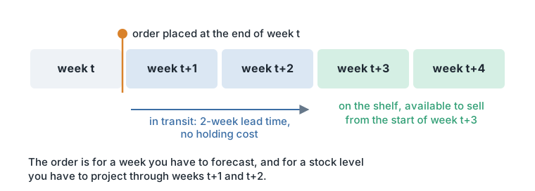
Sales are capped by the stock on the shelf, St = min(It, Dt), and unmet demand is lost, so every sales history we train on is censored demand. The score is the sum over weeks and series of 1.0 × lost sales + 0.2 × end-of-week stock.
Results
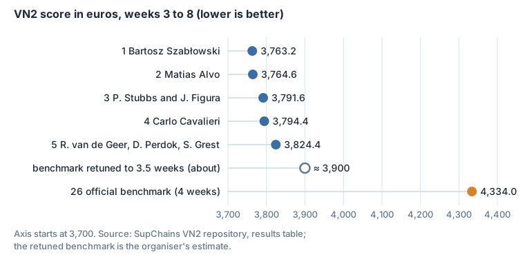
The official benchmark was a 13-week moving average with global seasonal factors, plus a flat 4-week stock target, in 55 lines of Python. It scored 4,334.0 €; the winner scored 3,763.2 €, 13.2% less. Vandeput, in his post-mortem: “The top 5 competitors beat the benchmark by an average of 13%. But only 25 participants (out of 180!) could beat it.”
Retuning the benchmark’s coverage from 4 weeks to about 3.5 weeks, changing one number and touching no model, would have scored about 3,900 € and ranked around 6th. Vandeput adds that the benchmark’s seasonal moving average turned out to be an accurate forecast, while its 4-week coverage was not optimised and was too long.
| # | Entrant | Approach | Score |
|---|---|---|---|
| 1 | Bartosz Szabłowski | Global CatBoost, direct multi-horizon, cost-aware order-up-to | 3,763.2 € |
| 2 | Matias Alvo | Deep reinforcement learning, the only participant to use it | 3,764.6 € |
| 3 | Philip Stubbs and Jakub Figura | 3,791.6 € | |
| 4 | Carlo Cavalieri | 3,794.4 € | |
| 5 | Ruben van de Geer, Diederik Perdok and Simon Grest | 3,824.4 € | |
| 26 | Official benchmark | 13-week seasonal moving average, 4-week stock target | 4,334.0 € |
Matias Alvo finished second, 1.4 € (0.04%) behind the winner.
The forecasting model
The winner trains one global CatBoost model jointly across all 599 series, with time series cast as tabular regression. It is direct multi-horizon: three independent models for h = 1, 2 and 3, each with the target shifted forward h weeks. It is trained with RMSE on the scaled target, with hyperparameters selected on MAE in original units. It is not recursive and does not use a Tweedie or Poisson loss, despite about 43% zero weeks: intermittency is handled by features.
CatBoost was compared with Random Forest and LightGBM on the same features and a comparable tuning budget, and the report states that performance is “tightly coupled to the feature engineering design”. Vandeput’s own tier list puts LightGBM in A-tier and CatBoost in B-tier.
Stockout-aware targets
A zero in a sales column means one of two different things: nobody wanted it, or there was none to sell. Train on both as if they were the same and the model learns that demand is lower than it is, then orders too little, which causes the next stockout. The paper masks those weeks:
y_eff_t = y_t    if in_stock_t = True
y_eff_t = NaN    otherwise          masked, not zero, not imputed to zero
Every target and every target-derived feature (lags, rolling means, medians, exponentially weighted means, std, IQR, momentum, slope) is computed on y_eff, not on raw sales.
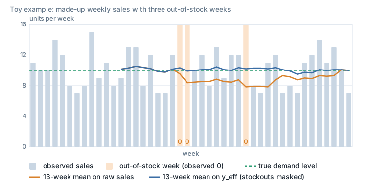
Masking leaves missing values, which the paper fills with the per-series median of scaled values, then the global one, rather than CatBoost’s native NaN handling, so that the model does not learn “out of stock” as a feature. The in-stock flag is only a likely shortage signal: Vandeput cautions that zero inventory at the end of a week does not prove lost sales.
Dynamic scaling
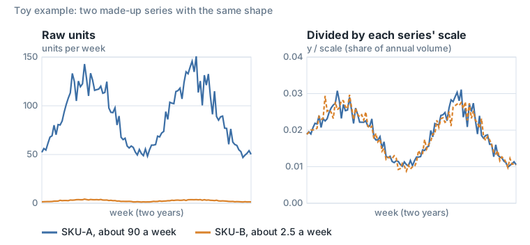
In a global model with a squared-error loss, high-volume series dominate the loss. The model then learns the level of each series more than its shape. VN2 series range from about 0.3 to about 99 units a week.
scale_t = max( 53 · mean_non-missing( y_eff_(t-52 ... t) ), 1 ) an annualised demand levelThe model is trained on y_eff / scale and its predictions are multiplied back by the scale. The 53-week mean needs at least 45 in-stock weeks; before that, the expanding mean is used. The scale is rolling, so it follows trend and lifecycle; it is computed on y_eff, so stockout weeks do not deflate it; clipping at 1 stops ultra-sparse series from dividing by about 0. It is applied to the target and to all target-based numeric features.
Recency weights
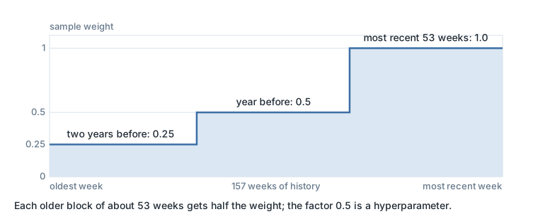
There is no differencing of the target. Drift is absorbed by dynamic scaling, change-based features (momentum, slope) and time-decayed sample weights: history is cut into blocks of about 53 weeks, the most recent block weighted 1.0, each older block halved. The decay factor is a hyperparameter; 0.5 is the value the report uses.
Features that describe each series
One model has to serve smooth high-volume items and lumpy long-tail items at the same time. The paper does not cluster them or learn embeddings. It uses categorical identity (store, product, series id, week of year), behavioural statistics (seasonality_strength, nonzero_rate, rolling std and IQR, momentum, time_since_spike), and dynamic scaling. The report notes that raw series-ID categoricals improve the leaderboard but do not generalise to a new store or product; in production it prefers stable parent-level categories.
Feature importance in the paper
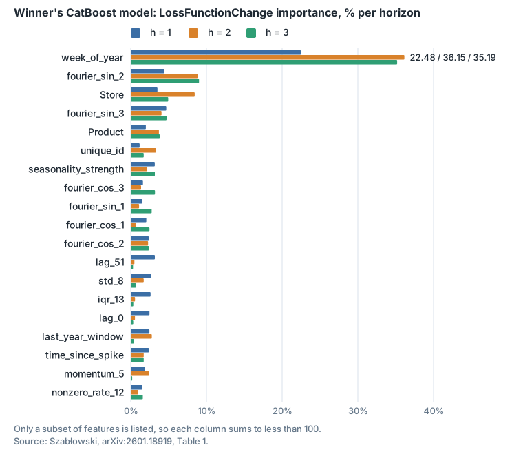
Calendar seasonality dominates, and its share grows from 22% at h=1 to 36% and 35% at h=2 and h=3, as recent lags lose predictive power.
The ordering policy
The order arrives after two more weeks of demand and two scheduled deliveries, so the policy first projects the stock to the delivery week from the forecasts. It then orders up to a target B = D̂t+3 + zq · φ · √D̂t+3, where zq = 0.9674 comes from the critical fractile q* = cs / (cs + ch) = 0.8333, and φ is calibrated by minimising the simulated total cost. Vandeput’s conclusion is that the top competitors stood out by their evaluation framework: they tested and tuned their policies by simulation.
VN2 features implementation
This was part of a review of our model’s base features, with the winner’s report as the source: arXiv:2601.18919.
Feature definition & implementation
Rolling level and dispersion features:
| Feature | Production definition |
|---|---|
rolling_mean_sales_3 | mean(xt−3, xt−2, xt−1) |
rolling_mean_sales_5 | mean(xt−5, …, xt−1) |
rolling_mean_sales_13 | mean(xt−13, …, xt−1) |
rolling_median_sales_3 | Approximate 50th percentile of xt−3…xt−1. |
rolling_median_sales_5 | Approximate 50th percentile of xt−5…xt−1. |
rolling_median_sales_13 | Approximate 50th percentile of xt−13…xt−1. |
rolling_std_sales_8 | Spark STDDEV over xt−8…xt−1. |
rolling_iqr_sales_13 | Approximate P75(xt−13…xt−1) − P25(xt−13…xt−1). |
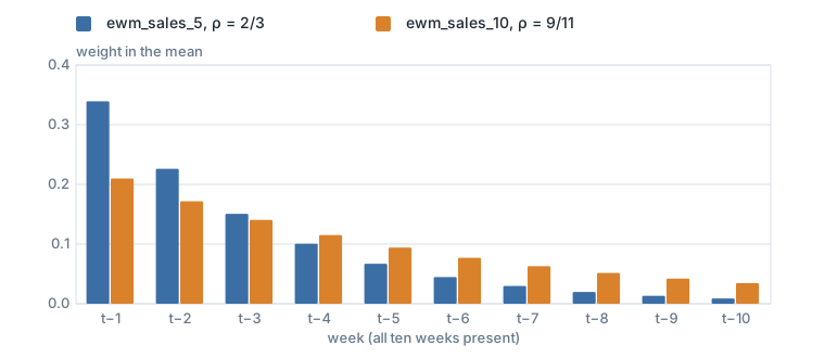
Exponentially weighted means: an exponentially weighted mean is a weighted average of recent sales. The most recent week gets the largest weight; each older week gets a smaller weight.
EWM_ρ(t) = [ Σ_(k=1…10) 1(x_(t−k) exists) × x_(t−k) × ρ^(k−1) ] / [ Σ_(k=1…10) 1(x_(t−k) exists) × ρ^(k−1) ]| Feature | Decay used in the code |
|---|---|
ewm_sales_5 | ρ = 0.6666666667 ≈ 2/3 |
ewm_sales_10 | ρ = 0.8181818182 ≈ 9/11 |
The two decays are the usual span convention, ρ = 1 − 2/(span + 1), the one pandas uses for spans 5 and 10.
Trend and demand-frequency features:
| Feature | Definition | What it is trying to describe |
|---|---|---|
momentum_sales_1 | xt−1 − xt−2 | Whether demand rose or fell from two weeks ago to last week. |
momentum_sales_5 | xt−1 − xt−6 | Whether last week was stronger or weaker than five weeks earlier. |
slope_sales_4 | (xt−1 − xt−5) / 4 | Average weekly direction of change during the previous four-week interval. |
nonzero_rate_sales_12 | Σk=1…12 1(xt−k > 0) / Σk=1…12 1(xt−k exists) | Actual behavior is the share of observed recent weeks that were above the series’ historical mean. |
Robust spike features
For the current week t:
- Look at sales from 2 to 14 weeks ago and take their median. This is the normal reference level mt.
- Estimate the typical amount by which historic sales differ from their own historic median. This is a robust variation measure dt, similar to a median absolute deviation (MAD).
- Take last week’s sales xt−1, subtract the normal reference, and divide by the typical variation.
robust_z_t = (last week's normalized sales − median) / MAD

weeks_since_spike(t) = [ date(t) − latest feature-row date(s) with robust_z(s) ≥ 3 ] / 7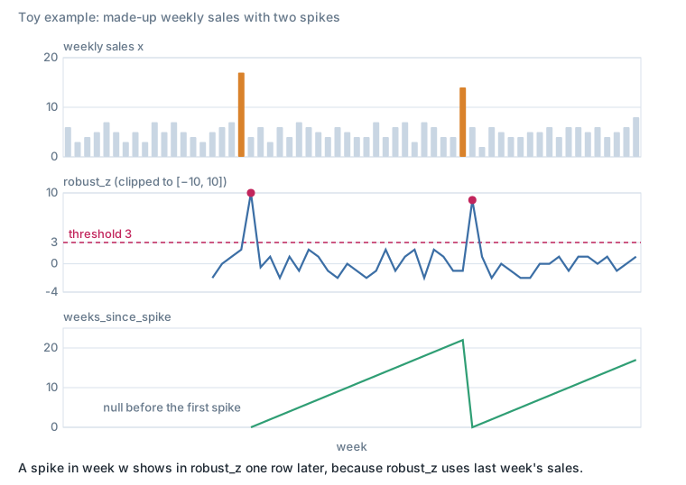
Intermittency score: rolling_mad_proxy / (rolling_median + 1)
Allows estimating how large the typical variation is compared with typical sales.
Seasonality strength
For each row r, define ar = xr−1 and br = xr−53. Then:
seasonality_strength_t = corr({a_r}, {b_r})where the production time window spans the preceding 364 days through the current row.
Fourier calendar features: coefficients and periods
x = weekofyear / 52
fourier_sin_k = sin(2π × k × weekofyear / 52)
fourier_cos_k = cos(2π × k × weekofyear / 52)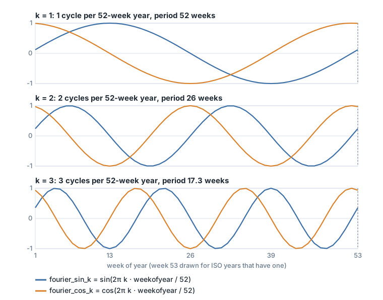
Because the code divides by 52, week 53 of an ISO year with 53 weeks gets the same values as week 1.
Feature correlation
Features are very correlated linearly.
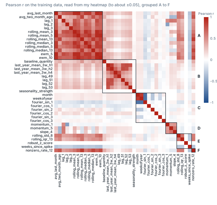
To effectively analyze the features and select only the relevant ones, we need to group them into meaningful categories:
| Group | Nature and members | Correlation interpretation |
|---|---|---|
| A, Recent sales level | avg_last_month_sales, avg_two_month_ago_sales, lags 1/2/3, rolling means 3/5/13, rolling medians 3/5/13, EWM-5, and EWM-10. | Directly comparable recent-demand summaries. This is the only group with super-correlated pairs. |
| B, Annual reference and seasonality | baseline_quantity, last-year centered means, annual lags 49/51/52/53, canonical H4 annual lag, and seasonality_strength. | Annual demand level and annual-repeat signal. |
| C, Calendar phase | month, weekofyear, Fourier sin/cos terms 1/2/3. | Functionally related calendar encodings. Pearson does not fully capture the nonlinear cyclic relationship between week number and sine/cosine. |
| D, Trend and momentum | Momentum 1/5 and slope 4. | Recent direction of demand change. |
| E, Variability and spikes | Rolling standard deviation, IQR, robust-z, and weeks since sales spike. | Demand volatility and abnormal-demand behavior. |
| F, Intermittency | nonzero_rate_sales_12. | Recent frequency of nonzero sales. |
| G, Static hierarchy and holiday | Store, country, three product hierarchy levels, and distance-to-holiday fields. | Categorical IDs are excluded from Pearson-correlation conclusions. |
Experiment
In development, on one product scope. Time to train models:
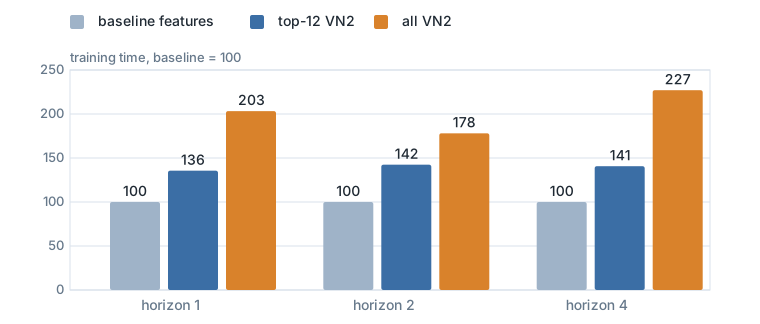
Selected features:
- ewm 5
- rolling std
- robust deviation
- weeks since spike
- cos and sin with period=52
- seasonality strength
SHAP analysis
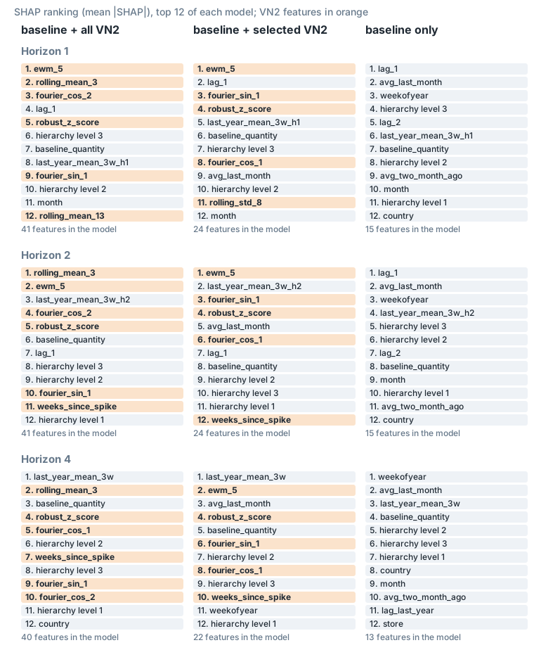
In the paper they kept woy and sin/cos (see the paper’s importance table in the background section).
Feature analysis
High seasonality should mean: if the last-year feature is high, the SHAP contribution of that feature is high. Meaning: pink points should be farther from the horizontal zero line than blue points, at comparable x-values.
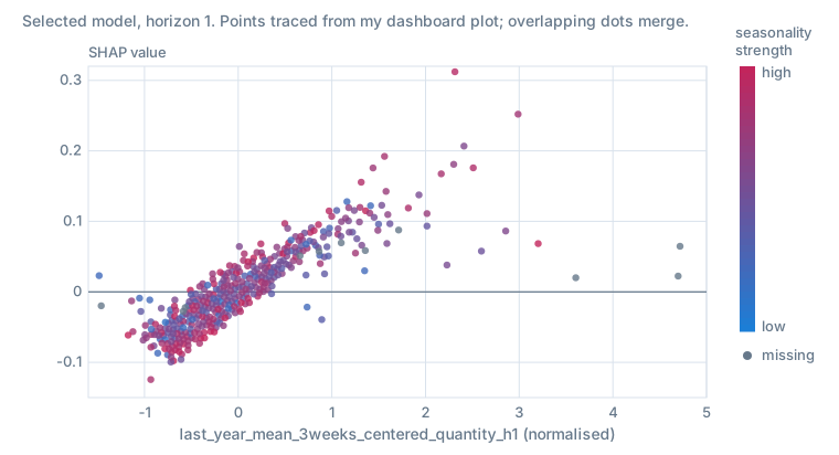
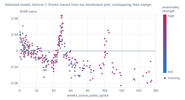
The highest contributions of weeks_since_sales_spike sit between about 45 and 52 weeks, about one year after the last spike.
Features:
- recent / last year: works well / as intended
- robust z score
- slow ewm baseline -> is it better than baseline_qtt? => it does contribute more
- weeks since last spike; doesn’t really contribute more
- momentum12 & momentum123 -> they do show up in the beeswarm as very important -> 12
- slope1? -> remove
- seasonality strength -> I should see low contribution of lag 51 or last year mean 3 weeks centered when the seasonality is low and high when the seasonality is high -> plot the SHAP dependence plot between their 2 features
- Split seasonality strength into low / medium / high groups, then plot a separate average or median SHAP curve for each group over the same last-year-sales bins, showing counts.
- rolling std sales qtt -> remove
- lag1/lag2/lag51 -> decide next time
- intermittency -> drop
- cos & sin: having only woy push as less than having cos & sin and woy -> so keep the 3?
Results of VN2 features integration backtesting
Optimization
Many experiments were conducted to see the effect of each feature independently. The goal of these experiments was to improve both Bias and RelMSE on sales quantity cohorts 2+ for 3 product scopes, each at its own cutoff week. Two other cutoff weeks were also checked. (RelMSE is the model’s mean squared error divided by the naive forecast’s.)
The results are as follows:
| Change tested | Did it work? |
|---|---|
| Remove Fourier features only | No |
| Remove seasonality strength only | No |
| Remove Fourier and seasonality strength together | Trade-off: better RelMSE, slightly worse absolute bias |
| Remove intermittency from the broad feature set | No |
| Replace the two-week slope with momentum | No: improved the broad parent, but not the baseline |
| Remove month, week, or both | No joint improvement |
| Add EWM or replace the baseline input with EWM | No: improved the broad parent, but not the baseline |
| Add the recent-to-last-year ratio only | Yes |
| Add the volatility, slope, robust-score and spike-age bundle | Yes: tested together, not individually |
| Use the clean recipe without Fourier, seasonality strength or intermittency | Yes: best result among the listed H1 candidates |
| Remove the ratio from the clean recipe | No |
| Other conditional momentum, intermittency and EWM variants | No joint improvement |
| Candidate | Absolute bias, against the classic baseline | RelMSE, against the classic baseline | Did it work? |
|---|---|---|---|
| Classic baseline | Reference | Reference | Reference |
| Baseline + ratio only | 2.8% smaller | 1.4% lower | Yes: modest improvement on both metrics |
| Baseline + clean early-feature bundle | 12.5% larger | 3.2% higher | No: both metrics worsened |
We decided to remove Fourier cos & sin because they showed no improvement compared with month & weekofyear.
The final optimized set of features decided on is:
H1-H3:
- rolling_std_sales_8
- slope_sales_2
- robust_z_score_sales
- weeks_since_sales_spike
- recent_to_last_year_ratio_h{h}
- seasonality_strength
H4:
- recent_to_last_year_ratio
- seasonality_strength
| Feature | Purpose | Horizons |
|---|---|---|
rolling_std_sales_8 | Sales volatility over the previous 8 weeks | H1-H3 |
slope_sales_2 | Sales at t-2 minus sales at t-1; negative means rising demand | H1-H3 |
robust_z_score_sales | Detect recent sales spikes using a historical median and robust deviation; clipped to [-10, 10] | H1-H3 |
weeks_since_sales_spike | Weeks since the latest robust score ≥ 3; null before the first spike | H1-H3 |
recent_to_last_year_ratio_h{h} | Recent 3-week mean versus horizon-aligned last-year mean, using raw sales and +1 smoothing | All |
seasonality_strength | Rolling 364-day correlation between recent and last-year demand, averaged across stores per country and product | All |
Backtesting
Some highlights.
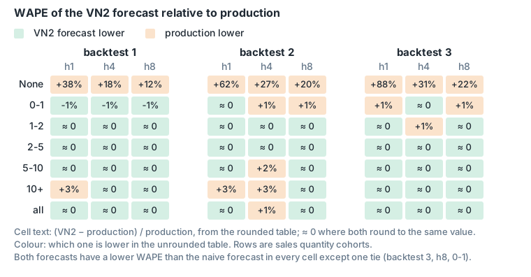
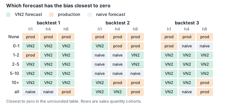
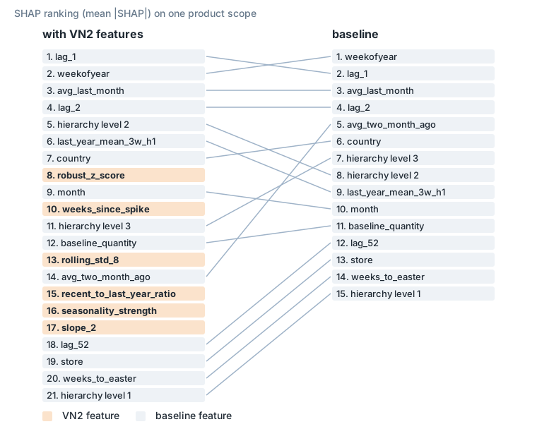
Beeswarm on one product scope, VN2 and baseline:
Conclusion
The metrics & viz show that the overall performance is better with VN2 features added. Although on a global scale it’s hard to see a huge improvement from these features, the explainability analysis done with our explainability dashboard shows examples where these added VN2 features make a clear difference in the outcome.
Sources
- Bartosz Szabłowski, One Global Model, Many Behaviors (VN2 Winner Report), arXiv:2601.18919, 2026.
- SupChains, VN2 repository: data, official simulator, benchmark and results.
- DataSource.ai, VN2 Inventory Planning Challenge, competition page (prizes).
- Nicolas Vandeput, My Learning Points from VN2, the First Inventory Competition (tier lists, benchmark retuning, the in-stock flag).
- SupChains, VN1 repository (VN1 score).
- pandas, DataFrame.ewm (span and decay).