These two studies follow the validation, hyperparameter and feature set studies on the same LightGBM model, which forecasts weekly sales per item and store with one model per product category x zone. The results are shown relative to the production model, as a difference in points (and, for RMSSE, an index where production is 100), not as absolute values.
Solve Bias Study
Executive Summary
During the last experiments (new training, new hyperparameters, new features), we have demonstrated multiple times that our model, as is, is unable to improve performance on high and low sellers simultaneously. In fact, when pushing the model in the direction of overfitting, we often observed an improved accuracy on low sellers and a worse bias on high sellers, which was due to the model prioritizing the majority class (low sellers) by reducing the forecasts overall.
This work aims to solve this core issue (unbalanced dataset) in 3 ways:
- Separation: separate models for the two classes, aka separate
- Initialization: different starting points for the two classes
- using the baseline quantity, aka init_baseline
- using the mean target, aka init_mean
- Normalization: transformation of the dataset to obtain a similar scale
- normalizing only the target, aka norm_t
- normalizing the target and features, aka norm_tf
As we observe in the results:
- These methods achieve significant improvement in performance and bias compared to the production models overall.
- The performance improvement varies significantly by model scope.
- Two methods take the lead: norm_tf and init_mean.
We demonstrate that these methods simultaneously improve the bias and accuracy on all significant cohorts, constituting a complete paradigm shift compared to recent experiments.
Introduction
The current model shows a performance imbalance when it comes to forecasting high sellers vs. low sellers. In particular, it over-forecasts low sellers and under-forecasts high sellers. This behaviour is illustrated below, when plotting the bias curve with respect to each selling class:
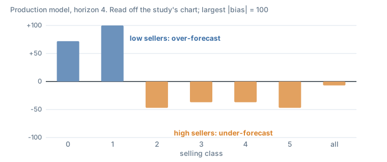
Figure 1. Bias by selling class of the production model, scaled so the largest absolute bias is 100.
In an attempt to mitigate this bias effect, we have investigated 3 different methods and compared the corresponding model performance using new cohorts and new metrics.
Presentation of Methods
Method 1: separate low sellers from high sellers
A first approach to mitigate the strong bias that is observed between low and high sellers consists in building two LightGBM models: 1 model for low sellers and 1 model for high sellers. The idea is to separate high and low selling articles directly in the training dataset. For each training set, a model is trained on the respective data.
The mean of sales quantities over all training history has been used to split the training dataset: a threshold of 1 has been selected (low sellers ”< 1” vs. high sellers ”>= 1”), supposedly splitting the articles in the proportions 20% (high sellers) / 80% (low sellers).
Note, 2 models vs. 1:
- a custom wrapper is handled the same way as a single model (no additional runs in production)
- the threshold to split the data becomes a hyperparameter that is hard to determine
Method 2: act on the model’s initialisation
Recall that LightGBM builds trees to compensate for errors from previously generated trees. In other words, LightGBM first initialises all sku/bu forecasts at a specific value. After initialisation, it starts building regression trees to “correct” errors made by this initial guess.
Roughly speaking, we can formulate the generated forecasts from LightGBM as:
LGBM_prediction(sku, bu) = init_score(sku, bu) + learning_rate x SUM[RegressionTreesCorrection(sku, bu, features)]After digging in the LightGBM documentation, we have noted that the model uses a common starting point for all sku/bu couples, which depends on the objective function. With the RMSE, forecasts are initialised using the mean over all sales targets (training dataset). With the Tweedie loss, forecasts are initialised using the log of the mean over all sales targets (training dataset). This is what LightGBM’s BoostFromScore does for the L2 and Tweedie objectives (source).
Since 80% of articles are sold less than 1 unit per week in the training dataset, the mean over all targets is close to 0. Hence, having an initial guess close to 0 for all articles has multiple consequences:
- LightGBM’s regression trees need to apply a larger correction for high sellers vs. low sellers (the latter already have a good initial forecast, whereas initial forecasts for high sellers are “far” from their true value): 0 is not a good initial guess for high sellers.
- LightGBM has to deal with separating high sellers from low sellers to handle the first point.
- Having a finite number of trees and a learning rate might cause LightGBM to stop before reaching appropriate convergence for high sellers, and might be partly responsible for the strong bias observed.
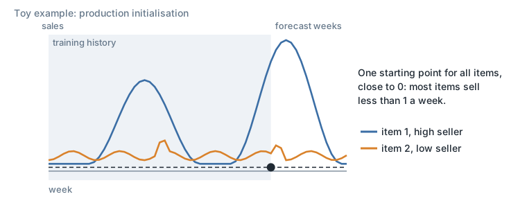
Figure 2. Initialisation in production. A toy example redrawn from the study’s sketch.
Therefore, providing a more appropriate initial guess for all articles (especially for high sellers) would reduce the amount of corrections the model needs to provide for high sellers. This simple initialisation trick could help the model better distinguish between low and high sellers, to bring the bias back closer to 0.
Two simple methods have been tested to estimate the initial guess:
- using the baseline quantity (rolling mean of sales quantities over the past 52 weeks) for each sku, bu and week (for a given sku/bu, the baseline quantity varies across weeks)
- using the mean of sales quantities over all available training history for each sku, bu (1 value for each sku/bu)
Note: articles with no history have been initialized at 0.
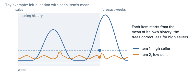
Figure 3. Initialisation using the mean of sales quantities. A toy example redrawn from the study’s sketch.
Method 3: normalise the data
A third approach consists in normalising the time series of the training dataset. By doing so, the model is fed with standardized signals with respect to each time series’ mean and standard deviation. This has two effects:
- LightGBM’s default initialisation is adapted for all standardized sku/bu (same effect as Method 2’s sku/bu specific initialisation). Note: the default initial guess is therefore the mean of sales quantities over all standardized samples. Since those samples are standardized, by definition they all have a mean at 0. Hence taking the mean over all standardized samples results in an initial guess at 0 for all sku/bu. Providing an initial estimate of 0 in the “standardized” world results in providing the mean as an initial guess in the “real” world for each individual sku/bu (same effect as Method 2’s sku/bu specific initialisation).
- Sales effects relative to sales quantities could be better understood by LightGBM, which now sees low, medium and high sellers on the same scale: low, medium and high sellers can be grouped in the same leaf if they have “similar” behaviour, hence the resulting forecast correction should be appropriately scaled relative to each time series, roughly “effects are proportional”.
Two methods have been investigated:
- normalize the sales quantity targets
- normalize the sales quantity targets and the sales related features
Both methods handle normalisation by subtracting the mean from the time series values and dividing by their respective standard deviation:
standardized_ts = (ts - mean(ts)) / std(ts)- ts: time series values (sales quantities or sales-related features)
- mean: average of values over all available training history, by sku/bu (similar value to Method 2’s mean of sales quantities)
- std: standard deviation of values over all available training history, by sku/bu
Note: articles with no history have no normalisation (impossibility).
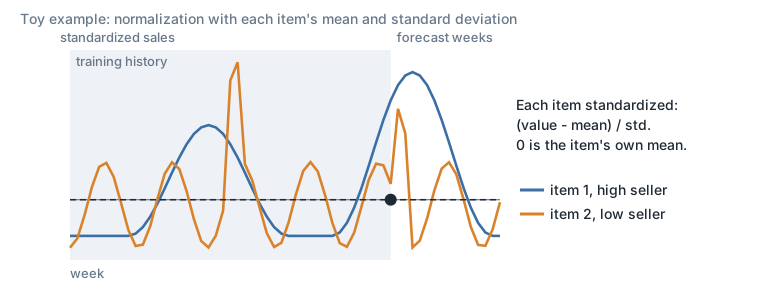
Figure 4. Normalisation using the mean and standard deviation. A toy example redrawn from the study’s sketch.
Experimental Setup
Summary of methods
| Method | Suffix |
|---|---|
| separate | separate |
| initialization | baseline quantity (init_baseline), mean (init_mean) |
| normalization | targets (norm_t), targets and features (norm_tf) |
Experiments scope
Two product category x zone perimeters, each with its own cutoff: perimeter A and perimeter B.
Results
The results are displayed compared to reconstructed sales; we observe similar patterns when comparing to sales quantity. All results are computed up to horizon 4.
All experiments
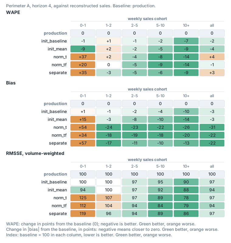
Figure 5. Perimeter A: WAPE, bias and volume-weighted RMSSE, relative to production, by weekly sales cohort.
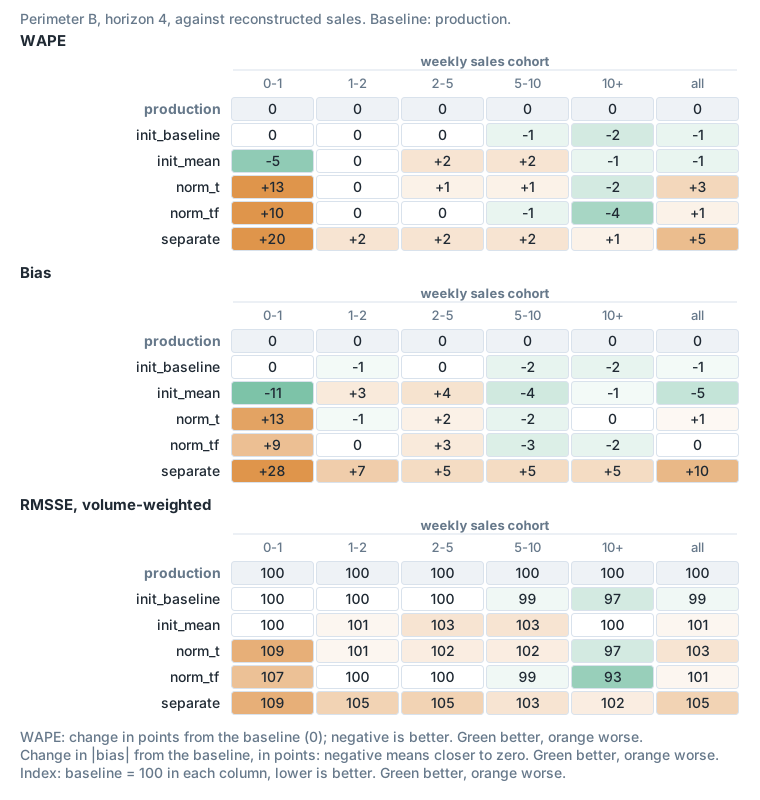
Figure 6. Perimeter B, the same comparison.
norm_t and init_baseline do offer better bias, but we believe this to be circumstantial.
We conclude that norm_tf and init_mean achieve the best overall consistency of results over performance and bias. They also are backed by theoretical evidence:
- Normalizing features as well as the target is known to improve performance.
- Having a fixed starting point instead of a variable one allows the model to have consistency.
We also note:
- init_baseline obtains better bias for perimeter B due to the fact that this cutoff is in a low season for the model scope, and therefore the baseline quantity is higher than the average.
Selected experiments
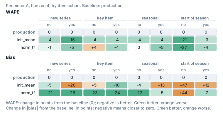
Figure 7. Perimeter A: WAPE and bias by new series, key items, seasonal items and start of seasonality, relative to production. The sales cohort results for init_mean and norm_tf are in Figure 5.
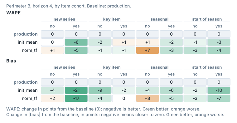
Figure 8. Perimeter B, the same comparison. The sales cohort results are in Figure 6.
We conclude that:
- results vary by model scope
- results are very encouraging: 10pts+ of WAPE improvement for high sellers and 20pts+ improvements of bias
- norm_tf achieves better performance for high sellers, while init_mean achieves better performance for low sellers
- norm_tf achieves better bias for perimeter A and init_mean for perimeter B
- norm_tf is more consistent (better RMSSE overall)
Dataset Normalization Study
Summary of findings
In our latest study (the solve bias study above), aiming at solving bias and the unbalanced dataset issue (low vs high sellers), we have shown very encouraging results for all methods tested. For the first time, we observe a significant improvement in both bias and accuracy.
Amongst the methods tested, one has shown the most improvement, which is normalization of target and features. In this work, we confirm these results with a wide backtesting of 3 cutoffs for multiple model scopes.
As we observe from the results:
- Normalization achieves significant improvement in performance and bias compared to the production models overall (from 2 to 10pts WAPE4 improvements and up to 25pts BIAS4 improvements).
- The performance improvement varies significantly by model scope (we notice in some cases some slight deterioration, mostly for low sellers, for cases of end of commercialization or for low history).
- From visualization examples, normalization shows great ability to reproduce seasonality. This is also apparent from the explainability analysis.
- From the explainability analysis, the model is much more capable of uncovering relationships between features.
Finally, we demonstrate that this method simultaneously improves the bias and accuracy on all significant cohorts, constituting a complete paradigm shift compared to recent experiments.
Intro and Setup of the Experimentation
Given the significant variability in observed previous results across different cutoffs and model scopes, a comprehensive and diversified backtesting process is required to ensure a proper evaluation of the solution.
- Code industrialisation: the code has been optimized:
- normalization taking place in the preprocessing
- denormalization taking place in the inference job
- Backtesting launch: the testing will be launched using Airflow DAGs for reliability and scale.
- Scope: backtesting will be conducted across all product category x zone combinations.
- Cutoffs: the evaluation will be performed on 3 specific cutoffs, cutoff 1, cutoff 2 and cutoff 3.
Evaluation and analysis:
- Metrics and cohorts: the results will be assessed using a set of new metrics and cohorts, complemented by visualizations.
- Forecasts comparison: the new forecasts will be explicitly analyzed against the production version.
- Metrics to be tracked (by cutoff):
- WAPE (Weighted Average Percentage Error)
- Bias
- WPE
- wRMSSE and wMASE, with volume as weight
- Cohorts for detailed assessment:
- product category x sales quantity
- product category x price range
- product category x key item
- product category x seasonal
- sales quantity cohorts
- turnover cohorts
- key item
- seasonal
- Visualizations: visualizations will be generated on different granularities, ensuring the inclusion of non-forecasted sales data.
Results
Metrics
The main takeaways by cutoff are:
Cutoff 1:
- 2pts improvement of WAPE4 across all sales and turnover cohorts
- Mostly improves “in seasonality” forecasts: start but also middle and end of season
- Improves both old and new time series
- Large improvements on product category C (8pts improvement of WAPE4 across high sales cohorts) and product category A (9pts improvement of WAPE4 across high sales cohorts and 15 to 20pts improvement of Bias4 across all sales cohorts except [0-1[)
- Other product categories are stable
Cutoff 2:
- 4pts improvement of WAPE4 across all sales and turnover cohorts
- 10pts improvement of WAPE4 for new time series
- Only improves “in seasonality” forecasts: start but also middle and end of season
- Large improvements on product category B (6pts improvement of WAPE4 across high sales cohorts) and product category A (9pts improvement of WAPE4 across high sales cohorts, but bias slightly deteriorated)
Cutoff 3:
- 2pts improvement of WAPE4 across all sales and turnover cohorts
- Mostly improves “in seasonality” forecasts: start but also middle and end of season
- Improves both old and new time series
- Large improvements on product category C (5pts improvement of WAPE4 across high sales cohorts and 8pts improvement of Bias4 across all sales cohorts except [0-1[) and product category D (7pts improvement of WAPE4 across high sales cohorts and 25pts improvement of Bias4 across all sales cohorts except [0-1[)
Visualization
We compared forecasts of the normalization model and the production model on individual series: the series where normalization achieves its best performance against the production model, neutral ones, and the ones where it achieves its worst. These charts show single products’ weekly sales, so they are not reproduced here.
One of the worst cases is an item that we kept because of our listing rule, although with the most up-to-date data we normally should not have forecast it. There is no stock data, which is why there are almost no sales.
Explainability
Example study
For the examples that displayed the worst performance of normalization, we’ve conducted an explainability analysis of the normalized model, which shows that:
- The main reason for the low forecast is the absence of lag 52.
- The normalized model doesn’t rely on lag 1 and lag 2, contrary to the production model.
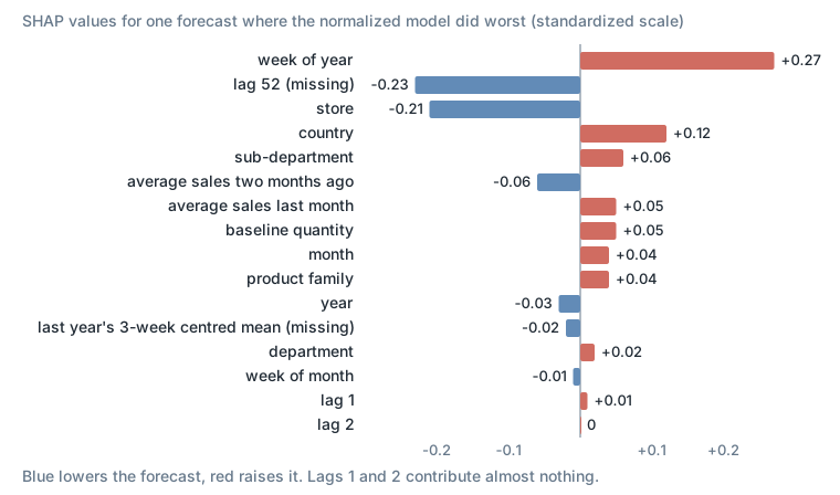
Figure 9. Contributions to one forecast where the normalized model did worst. SHAP values are in the model’s standardized output units, not an accuracy metric.
Distribution shift
Example of the distribution of the baseline quantity before and after normalization:
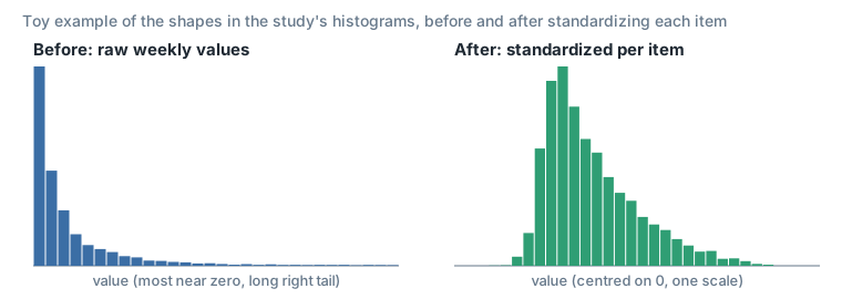
Figure 10. A toy example with the shapes of the study’s two histograms, made-up data.
Beeswarm plot
- The model trained on normalized features is less sensitive to recent lags.
- For the normalized features, the transition between negative and positive effect on the model is smoothly correlated to the value of the feature.
- The normalized model relies much less on recent sales (lag 1 and lag 2), and more on week of year and the lag of last year.
Features impact on the model
After normalization:
- The relationships between different features are more apparent to the model, which allows the uncovering of more complex relationships.
- The effect on the model is more balanced (almost half of the points have a positive impact and the other half a negative impact, on the scale of SHAP).
- The transition between negative and positive SHAP values is more smoothly correlated to the distribution of the feature.
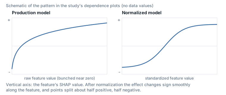
Figure 11. A schematic of the pattern in the study’s dependence plots, without data values.
Conclusion
As we observe from the results:
- Normalization achieves significant improvement in performance and bias compared to the production models overall (an average of 3pts and up to 10pts WAPE4 improvements, and up to 25pts BIAS4 improvements).
- The performance improvement varies significantly by model scope (we notice in some cases some slight deterioration, mostly for low sellers, end of commercialization or low history).
- The normalized model relies much less on recent sales (lag 1 and lag 2) and more on week of year, baseline quantity and the lag of last year.
- The model is able to better uncover complex relationships between features after normalization.
When there is an improvement, normalization simultaneously improves the bias and accuracy on all significant cohorts, constituting a complete paradigm shift compared to recent experiments.
Next steps
- After the positive results during backtesting, the dataset normalization will be deployed to production in the upcoming weeks.
- Normalization also opens up new possibilities. We have seen from the explainability analysis that our model is much more capable of discovering relationships between different features. Moreover, non-sales related features appear to contribute to the model’s performance. Therefore, we’d like to revisit some of the features we’ve tried introducing in the past (price, sku/bu, calendar, weather, …).
- Normalization can also simplify the cold start process. In fact, we simply improve the forecast for new (sku, bu) by using the (mean, std) derived from similar items to denormalize predictions during the inference.
- As this new modeling method achieves a major step forward, we would like to quantify the improvement from a business perspective. We want to use turnover information to conduct an analysis of the potential gains unlocked with the better forecast provided by this method:
- use turnover cohorts
- use accuracy
- focus on key sellers (ABC classes? selling class? turnover cohorts? 5-40 / 20-80? key items?)